The paper discusses a conceptually challenging issue in cosmology, which I’ll put simply as follows. Suppose we have two cosmological theories: A, which describes a very large universe in only a tiny part of which low-energy physics turns out like ours; and B in which we have a possibly much smaller universe in which low-energy physics is like ours with a high probability. Can we determine whether A or B is the “better” theory, and if so how?
The abstract of the paper is below:
Some cosmological theories propose that the observable universe is a small part of a much larger universe in which parameters describing the low-energy laws of physics vary from region to region. How can we reasonably assess a theory that describes such a mostly unobservable universe? We propose a Bayesian method based on theory-generated probability distributions for our observations. We focus on basic principles, leaving aside concerns about practicality. (We also leave aside the measure problem, to discuss other issues.) We argue that cosmological theories can be tested by standard Bayesian updating, but we need to use theoretical predictions for “first-person” probabilities — i.e., probabilities for our observations, accounting for all relevant selection effects. These selection effects can depend on the observer, and on time, so in principle first-person probabilities are defined for each observer-instant — an observer at an instant of time. First-person probabilities should take into account everything the observer believes about herself and her surroundings — i.e., her “subjective state”. We advocate a “Principle of Self-Locating Indifference” (PSLI), asserting that any real observer should make predictions as if she were chosen randomly from the theoretically predicted observer-instants that share her subjective state. We believe the PSLI is intuitively very reasonable, but also argue that it maximizes the expected fraction of observers who will make correct predictions. Cosmological theories will in general predict a set of possible universes, each with a probability. To calculate first-person probabilities, we argue that each possible universe should be weighted by the number of observer-instants in the specified subjective state that it contains. We also discuss Boltzmann brains, the humans/Jovians parable of Hartle and Srednicki, and the use of “old evidence”.
arXiv:2602.02667
I haven’t had time to read the paper in detail yet, and I don’t think I’m going to agree with all of it when I do, but I found it sufficiently stimulating to share here in the hope that others will find it interesting.
I got an email last week pointing out that I had won another prize in the Times Literary Supplement crossword competition 1565. They have modernised at the TLS, so instead of sending a cheque for the winnings, they pay by bank transfer and wanted to check whether my details had changed since last time. You can submit by email nowadays too, which saves a bit in postage.
Anyway, I checked this week’s online edition and found this for proof:
I checked when I last won this competition, which I enter just about every week, and found that it was number 1514, almost exactly a year ago. There are 50 competitions per year rather than 52, because there are double issues at Christmas and in August, so it’s actually just over a year (51 puzzles) since I last won. I’ve won the crossword prize quite a few times but haven’t been very careful at keeping track of the dates. I think it’s been about once a year since I started entering.
All this suggested to me a little problem I devised when I was teaching probability and statistics many years ago:
Let’s assume that the same number of correct entries, N, is submitted for each competition. The winner each time is drawn randomly from among these N. If there are 50 competitions in a year and I submit a correct answer each time, winning once in these 50 submissions, then what can I infer about N?
Answers on a postcard, via email, or, preferably, via the Comments!
Here’s an interestingly different talk in the series of Cosmology Talks curated by Shaun Hotchkiss. The speaker, Sylvia Wenmackers, is a philosopher of science. According to the blurb on Youtube:
Her focus is probability and she has worked on a few theories that aim to extend and modify the standard axioms of probability in order to tackle paradoxes related to infinite spaces. In particular there is a paradox of the “infinite fair lottery” where within standard probability it seems impossible to write down a “fair” probability function on the integers. If you give the integers any non-zero probability, the total probability of all integers is unbounded, so the function is not normalisable. If you give the integers zero probability, the total probability of all integers is also zero. No other option seems viable for a fair distribution. This paradox arises in a number of places within cosmology, especially in the context of eternal inflation and a possible multiverse of big bangs bubbling off. If every bubble is to be treated fairly, and there will ultimately be an unbounded number of them, how do we assign probability? The proposed solutions involve hyper-real numbers, such as infinitesimals and infinities with different relative sizes, (reflecting how quickly things converge or diverge respectively). The multiverse has other problems, and other areas of cosmology where this issue arises also have their own problems (e.g. the initial conditions of inflation); however this could very well be part of the way towards fixing the cosmological multiverse.
The paper referred to in the presentation can be found here. There is a lot to digest in this thought-provoking talk, from the starting point on Kolmogorov’s axioms to the application to the multiverse, but this video gives me an excuse to repeat my thoughts on infinities in cosmology.
Most of us – whether scientists or not – have an uncomfortable time coping with the concept of infinity. Physicists have had a particularly difficult relationship with the notion of boundlessness, as various kinds of pesky infinities keep cropping up in calculations. In most cases this this symptomatic of deficiencies in the theoretical foundations of the subject. Think of the ‘ultraviolet catastrophe‘ of classical statistical mechanics, in which the electromagnetic radiation produced by a black body at a finite temperature is calculated to be infinitely intense at infinitely short wavelengths; this signalled the failure of classical statistical mechanics and ushered in the era of quantum mechanics about a hundred years ago. Quantum field theories have other forms of pathological behaviour, with mathematical components of the theory tending to run out of control to infinity unless they are healed using the technique of renormalization. The general theory of relativity predicts that singularities in which physical properties become infinite occur in the centre of black holes and in the Big Bang that kicked our Universe into existence. But even these are regarded as indications that we are missing a piece of the puzzle, rather than implying that somehow infinity is a part of nature itself.
The exception to this rule is the field of cosmology. Somehow it seems natural at least to consider the possibility that our cosmos might be infinite, either in extent or duration, or both, or perhaps even be a multiverse comprising an infinite collection of sub-universes. If the Universe is defined as everything that exists, why should it necessarily be finite? Why should there be some underlying principle that restricts it to a size our human brains can cope with?
On the other hand, there are cosmologists who won’t allow infinity into their view of the Universe. A prominent example is George Ellis, a strong critic of the multiverse idea in particular, who frequently quotes David Hilbert
The final result then is: nowhere is the infinite realized; it is neither present in nature nor admissible as a foundation in our rational thinking—a remarkable harmony between being and thought
But to every Hilbert there’s an equal and opposite Leibniz
I am so in favor of the actual infinite that instead of admitting that Nature abhors it, as is commonly said, I hold that Nature makes frequent use of it everywhere, in order to show more effectively the perfections of its Author.
You see that it’s an argument with quite a long pedigree!
Many years ago I attended a lecture by Alex Vilenkin, entitled The Principle of Mediocrity. This was a talk based on some ideas from his book Many Worlds in One: The Search for Other Universes, in which he discusses some of the consequences of the so-called eternal inflation scenario, which leads to a variation of the multiverse idea in which the universe comprises an infinite collection of causally-disconnected “bubbles” with different laws of low-energy physics applying in each. Indeed, in Vilenkin’s vision, all possible configurations of all possible things are realised somewhere in this ensemble of mini-universes.
One of the features of this scenario is that it brings the anthropic principle into play as a potential “explanation” for the apparent fine-tuning of our Universe that enables life to be sustained within it. We can only live in a domain wherein the laws of physics are compatible with life so it should be no surprise that’s what we find. There is an infinity of dead universes, but we don’t live there.
I’m not going to go on about the anthropic principle here, although it’s a subject that’s quite fun to write or, better still, give a talk about, especially if you enjoy winding people up! What I did want to say mention, though, is that Vilenkin correctly pointed out that three ingredients are needed to make this work:
An infinite ensemble of realizations
A discretizer
A randomizer
Item 2 involves some sort of principle that ensures that the number of possible states of the system we’re talking about is not infinite. A very simple example from quantum physics might be the two spin states of an electron, up (↑) or down(↓). No “in-between” states are allowed, according to our tried-and-tested theories of quantum physics, so the state space is discrete. In the more general context required for cosmology, the states are the allowed “laws of physics” ( i.e. possible false vacuum configurations). The space of possible states is very much larger here, of course, and the theory that makes it discrete much less secure. In string theory, the number of false vacua is estimated at 10500. That’s certainly a very big number, but it’s not infinite so will do the job needed.
Item 3 requires a process that realizes every possible configuration across the ensemble in a “random” fashion. The word “random” is a bit problematic for me because I don’t really know what it’s supposed to mean. It’s a word that far too many scientists are content to hide behind, in my opinion. In this context, however, “random” really means that the assigning of states to elements in the ensemble must be ergodic, meaning that it must visit the entire state space with some probability. This is the kind of process that’s needed if an infinite collection of monkeys is indeed to type the (large but finite) complete works of shakespeare. It’s not enough that there be an infinite number and that the works of shakespeare be finite. The process of typing must also be ergodic.
Now it’s by no means obvious that monkeys would type ergodically. If, for example, they always hit two adjoining keys at the same time then the process would not be ergodic. Likewise it is by no means clear to me that the process of realizing the ensemble is ergodic. In fact I’m not even sure that there’s any process at all that “realizes” the string landscape. There’s a long and dangerous road from the (hypothetical) ensembles that exist even in standard quantum field theory to an actually existing “random” collection of observed things…
More generally, the mere fact that a mathematical solution of an equation can be derived does not mean that that equation describes anything that actually exists in nature. In this respect I agree with Alfred North Whitehead:
There is no more common error than to assume that, because prolonged and accurate mathematical calculations have been made, the application of the result to some fact of nature is absolutely certain.
It’s a quote I think some string theorists might benefit from reading!
Items 1, 2 and 3 are all needed to ensure that each particular configuration of the system is actually realized in nature. If we had an infinite number of realizations but with either infinite number of possible configurations or a non-ergodic selection mechanism then there’s no guarantee each possibility would actually happen. The success of this explanation consequently rests on quite stringent assumptions.
I’m a sceptic about this whole scheme for many reasons. First, I’m uncomfortable with infinity – that’s what you get for working with George Ellis, I guess. Second, and more importantly, I don’t understand string theory and am in any case unsure of the ontological status of the string landscape. Finally, although a large number of prominent cosmologists have waved their hands with commendable vigour, I have never seen anything even approaching a rigorous proof that eternal inflation does lead to realized infinity of false vacua. If such a thing exists, I’d really like to hear about it!
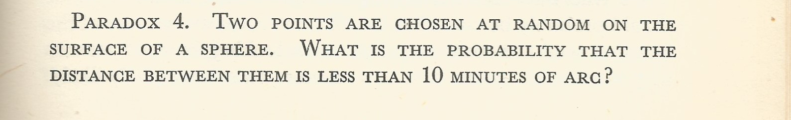
I just came across this paradox in an old book of mathematical recreations and thought it was cute so I’d share it here:
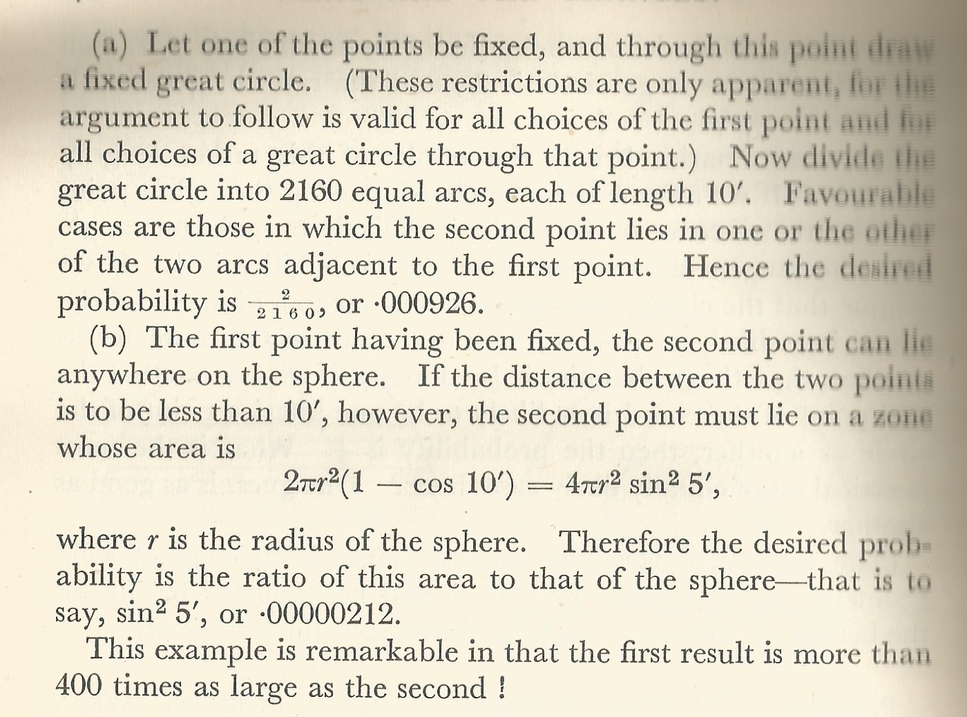
Here are two possible solutions to pick from:
Since we are now in the era of precision cosmology, an uncertainty of a factor of 400 is not acceptable so which answer is correct? Or are they both wrong?
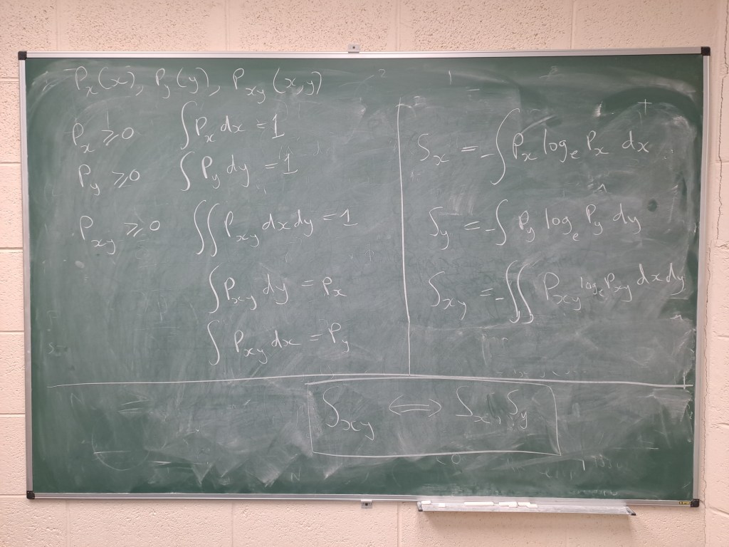
I thought I’d use the medium of this blog to pick the brains of my readers about some general questions I have about probability and entropy as described on the chalkboard above in order to help me with my homework.
Imagine that px(x) and py(y) are one-point probability density functions and pxy(x,y) is a two-point (joint) probability density function defined so that its marginal distributions are px(x) and py(y) and shown on the left-hand side of the board. These functions are all non-negative definite and integrate to unity as shown.
Note that, unless x and y are independent, in which case pxy(x,y) = px(x) py(y), the joint probability cannot be determined from the marginals alone.
On the right we have Sx, Sy and Sxy defined by integrating plogp for the two univariate distributions and the bivariate distributions respectively as shown on the right-hand side of the board. These would be proportional to the Gibbs entropy of the distributions concerned but that isn’t directly relevant.
My question is: what can be said in general terms (i.e. without making any further assumptions about the distributions involved) about the relationship between Sx, Sy and Sxy ?
Answers on a postcard through the comments block please!
I have been struck by the number of people upset by the latest analysis of SARS-Cov-2 “variants of concern” byPublic Health England. In particular it is in the report that over 40% of those dying from the so-called Delta Variant have had both vaccine jabs. I even saw some comments on social media from people saying that this proves that the vaccines are useless against this variant and as a consequence they weren’t going to bother getting their second jab.
This is dangerous nonsense and I think it stems – as much dangerous nonsense does – from a misunderstanding of basic probability which comes up in a number of situations, including the Prosecutor’s Fallacy. I’ll try to clarify it here with a bit of probability theory. The same logic as the following applies if you specify serious illness or mortality, but I’ll keep it simple by just talking about contracting Covid-19. When I write about probabilities you can think of these as proportions within the population so I’ll use the terms probability and proportion interchangeably in the following.
Denote by P[C|V] the conditional probability that a fully vaccinated person becomes ill from Covid-19. That is considerably smaller than P[C| not V] (by a factor of ten or so given the efficacy of the vaccines). Vaccines do not however deliver perfect immunity so P[C|V]≠0.
Let P[V|C] be the conditional probability of a person with Covid-19 having been fully vaccinated. Or, if you prefer, the proportion of people with Covid-19 who are fully vaccinated..
Now the first thing to point out is that these conditional probability are emphatically not equal. The probability of a female person being pregnant is not the same as the probability of a pregnant person being female.
We can find the relationship between P[C|V] and P[V|C] using the joint probability P[V,C]=P[V,C] of a person having been fully vaccinated and contracting Covid-19. This can be decomposed in two ways: P[V,C]=P[V]P[C|V]=P[C]P[V|C]=P[V,C], where P[V] is the proportion of people fully vaccinated and P[C] is the proportion of people who have contracted Covid-19. This gives P[V|C]=P[V]P[C|V]/P[C].
This result is nothing more than the famous Bayes Theorem.
Now P[C] is difficult to know exactly because of variable testing rates and other selection effects but is presumably quite small. The total number of positive tests since the pandemic began in the UK is about 5M which is less than 10% of the population. The proportion of the population fully vaccinated on the other hand is known to be about 50% in the UK. We can be pretty sure therefore that P[V]»P[C]. This in turn means that P[V|C]»P[C|V].
In words this means that there is nothing to be surprised about in the fact that the proportion of people being infected with Covid-19 is significantly larger than the probability of a vaccinated person catching Covid-19. It is expected that the majority of people catching Covid-19 in the current phase of the pandemic will have been fully vaccinated.
(As a commenter below points out, in the limit when everyone has been vaccinated 100% of the people who catch Covid-19 will have been vaccinated. The point is that the number of people getting ill and dying will be lower than in an unvaccinated population.)
The proportion of those dying of Covid-19 who have been fully vaccinated will also be high, a point also made here.
It’s difficult to be quantitatively accurate here because there are other factors involved in the risk of becoming ill with Covid-19, chiefly age. The reason this poses a problem is that in my countries vaccinations have been given preferentially to those deemed to be at high risk. Younger people are at relatively low risk of serious illness or death from Covid-19 whether or not they are vaccinated compared to older people, but the latter are also more likely to have been vaccinated. To factor this into the calculation above requires an additional piece of conditioning information. We could express this crudely in terms of a binary condition High Risk (H) or Low Risk (L) and construct P(V|L,H) etc but I don’t have the time or information to do this.
So please don’t be taken in by this fallacy. Vaccines do work. Get your second jab (or your first if you haven’t done it yet). It might save your life.
A test is designed to show whether or not a person is carrying a particular virus.
The test has only two possible outcomes, positive or negative.
If the person is carrying the virus the test has a 95% probability of giving a positive result.
If the person is not carrying the virus the test has a 95% probability of giving a negative result.
A given individual, selected at random, is tested and obtains a positive result. What is the probability that they are carrying the virus?
Update 1: the comments so far have correctly established that the answer is not what you might naively think (ie 95%) and that it dependson the fraction of people in the population actually carrying the virus. Suppose this is f. Now what is the answer?
Update 2: OK so we now have the probability for a fixed value of f. Suppose we know nothing about f in advance. Can we still answer the question?
Answers and/or comments through the comments box please.
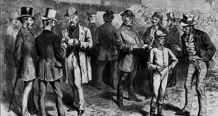
I read an interesting piece in Sunday’s Observer which is mainly about the challenges facing the modern sports betting industry but which also included some interesting historical snippets about the history of gambling.
One thing that I didn’t know before reading this article was that it is generally accepted that the first ever bookmaker was a chap called Harry Ogden who started business in the late 18th century on Newmarket Heath. Organized horse-racing had been going on for over a century by then, and gambling had co-existed with it, not always legally. Before Harry Ogden, however, the types of wager were very different from what we have nowadays. For one thing bets would generally be offered on one particular horse (the Favourite), against the field. There being only two outcomes these were generally even-money bets, and the wagers were made between individuals rather than being administered by a `turf accountant’.
Then up stepped Harry Ogden, who introduced the innovation of laying odds on every horse in a race. He set the odds based on his knowledge of the form of the different horses (i.e. on their results in previous races), using this data to estimate probabilities of success for each one. This kind of `book’, listing odds for all the runners in a race, rapidly became very popular and is still with us today. The way of specifying odds as fractions (e.g. 6/1 against, 7/1 on) derives from this period.
Ogden wasn’t interested in merely facilitating other people’s wagers: he wanted to make a profit out of this process and the system he put in place to achieve this survives to this day. In particular he introduced a version of the overround, which works as follows. I’ll use a simple example from football rather than horse-racing because I was thinking about it the other day while I was looking at the bookies odds on relegation from the Premiership.
Suppose there is a football match, which can result either in a HOME win, an AWAY win or a DRAW. Suppose the bookmaker’s expert analysts – modern bookmakers employ huge teams of these – judge the odds of these three outcomes to be: 1-1 (evens) on a HOME win, 2-1 against the DRAW and 5-1 against the AWAY win. The corresponding probabilities are: 1/2 for the HOME win, 1/3 for the DRAW and 1/6 for the AWAY win. Note that these add up to 100%, as they are meant to be probabilities and these are the only three possible outcomes. These are `true odds’.
Offering these probabilities as odds to punters would not guarantee a return for the bookie, who would instead change the odds so they add up to more than 100%. In the case above the bookie’s odds might be: 4-6 for the HOME win; 6-4 for the DRAW and 4-1 against the AWAY win. The implied probabilities here are 3/5, 2/5 and 1/5 respectively, which adds up to 120%, not 100%. The excess is the overround or `bookmaker’s margin’ – in this case 20%.
This is quite the opposite to the Dutch Book case I discussed here.
Harry Ogden applied his method to horse races with many more possible outcomes, but the principle is the same: work out your best estimate of the true odds then apply your margin to calculate the odds offered to the punter.
One thing this means is that you have to be careful f you want to estimate the probability of an event from a bookie’s odds. If they offer you even money then that does not mean they you have a 50-50 chance!
I’m posting this in the Cute Problems folder, but I’m mainly putting it up here as a sort of experiment. This little puzzle was posted on Twitter by someone I follow and it got a huge number of responses (>25,000). I was fascinated by the replies, and I’m really interested to see whether the distribution of responses from readers of this blog is different.
Anyway, here it is, exactly as posted on Twitter:
Assume there is a 50:50 chance of any child being male or female.
Now assume four generations, all other things being equal.
What are the odds of a son being a son of a son of a son?
Last week, realizing that it had been a while since I posted anything in the cute problems folder, I did a quick post before going to a meeting. Unfortunately, as a couple of people pointed out almost immediately, there was a problem with the question (a typo in the form of a misplaced bracket). I took the post offline until I could correct it and then promptly forgot about it. I remembered it yesterday so have now corrected it. I also added a useful integral as a hint at the end, because I’m a nice person. I suggest you start by evaluating the expectation value (i.e. the first-order moment). Answers to parts (2) and (3) through the comments box please!
Answers to (2) and (3) via the comments box please!
SOLUTION: I’ll leave you to draw your own sketch but, as Anton correctly points out, this is a distribution that is asymmetric about its mean but has all odd-order moments equal (including the skewness) equal to zero. it therefore provides a counter-example to common assertions, e.g. that asymmetric distributions must have non-zero skewness. The function shown in the problem was originally given by Stieltjes, but a general discussion can be be found in E. Churchill (1946) Information given by odd moments, Ann. Math. Statist. 17, 244-6. The paper is available online here.
The views presented here are personal and not necessarily those of my employer (or anyone else for that matter).
Feel free to comment on any of the posts on this blog but comments may be moderated; anonymous comments and any considered by me to be vexatious and/or abusive and/or defamatory will not be accepted. I do not necessarily endorse, support, sanction, encourage, verify or agree with the opinions or statements of any information or other content in the comments on this site and do not in any way guarantee their accuracy or reliability.