The era of modern physics could be said to have begun in 1687 with the publication by Sir Isaac Newton of his great Philosophiae Naturalis Principia Mathematica, (Principia for short). In this magnificent volume, Newton presented a mathematical theory of all known forms of motion and, for the first time, gave clear definitions of the concepts of force and momentum. Within this general framework he derived a new theory of Universal Gravitation and used it to explain the properties of planetary orbits previously discovered but unexplained by Johannes Kepler. The classical laws of motion and his famous “inverse square law” of gravity have been superseded by more complete theories when dealing with very high speeds or very strong gravity, but they nevertheless continue supply a very accurate description of our everyday physical world.
Newton’s laws have a rigidly deterministic structure. What I mean by this is that, given precise information about the state of a system at some time then one can use Newtonian mechanics to calculate the precise state of the system at any later time. The orbits of the planets, the positions of stars in the sky, and the occurrence of eclipses can all be predicted to very high accuracy using this theory.
At this point it is useful to mention that most physicists do not use Newton’s laws in the form presented in the Principia, but in a more elegant language named after Sir William Rowan Hamilton. The point about Newton’s laws of motion is that they are expressed mathematically as differential equations: they are expressed in terms of rates of changes of things. For instance, the force on a body gives the rate of change of the momentum of the body. Generally speaking, differential equations are very nasty things to solve which is a shame because most a great deal of theoretical physics involves them. Hamilton realised that it was possible to express Newton’s laws in a way that did not involve clumsy mathematics of this type. His formalism was equivalent, in the sense that one could obtain the basic differential equations from it, but easier to use in general situations. The key concept he introduced – now called the Hamiltonian – is a single mathematical function that depends on both the positions q and momenta p of the particles in a system, say H(q,p). This function is constructed from the different forms of energy (kinetic and potential) in the system, and how they depend on the p’s and q’s, but the details of how this works out don’t matter. Suffice to say that knowing the Hamiltonian for a system is tantamount to a full classical description of its behaviour.
Hamilton was a very interesting character. He was born in Dublin in 1805 and showed an astonishing early flair for languages, speaking 13 of them by the time he was 13. He graduated from Trinity College aged 22, at which point he was clearly a whiz-kid at mathematics as well as languages. He was immediately made professor of astronomy at Dublin and Astronomer Royal for Ireland. However, he turned out to be hopeless at the practicalities of observational work. Despite employing three of his sisters to help him in the observatory he never produced much of astronomical interest. Mathematics and alcohol seem to have been the two real loves of his life.
It is a fascinating historical fact that the development of probability theory during the late 17th and early 18th century coincided almost exactly with the rise of Newtonian Mechanics. It may seem strange in retrospect that there was no great philosophical conflict between these two great intellectual achievements since they have mutually incompatible views of prediction. Probability applies in unpredictable situations; Newtonian Mechanics says that everything is predictable. The resolution of this conundrum may owe a great deal to Laplace, who contributed greatly to both fields. Laplace, more than any other individual, was responsible to elevated the deterministic world-view of Newton to a scientific principle in its own right. To quote:
We ought then to regard the present state of the Universe as the effect of its preceding state and as the cause of its succeeding state.
According to Laplace’s view, knowledge of the initial conditions pertaining at the instant of creation would be sufficient in order to predict everything that subsequently happened. For him, a probabilistic treatment of phenomena did not conflict with classical theory, but was simply a convenient approach to be taken when the equations of motion were too difficult to be solved exactly. The required probabilities could be derived from the underlying theory, perhaps using some kind of symmetry argument.
The s-called “randomizing” devices used in all traditional gambling games – roulette wheels, dice, coins, bingo machines, and so on – are in fact well described by Newtonian mechanics. We call them “random” because the motions involved are just too complicated to make accurate prediction possible. Nevertheless it is clear that they are just straightforward mechanical devices which are essentially deterministic. On the other hand, we like to think the weather is predictable, at least in principle, but with much less evidence that it is so!
But it is not only systems with large numbers of interacting particles (like the Earth’s atmosphere) that pose problems for predictability. Some deceptively simple systems display extremely erratic behaviour. The theory of these systems is less than fifty years old or so, and it goes under the general title of nonlinear dynamics. One of the most important landmarks in this field was a study by two astronomers, Michel Hénon and Carl Heiles in 1964. They were interested in what would happens if you take a system with a known analytical solutions and modify it.
In the language of Hamiltonians, let us assume that H0 describes a system whose evolution we know exactly and H1 is some perturbation to it. The Hamiltonian of the modified system is thus

What Hénon and Heiles did was to study a system whose unmodified form is very familiar to physicists: the simple harmonic oscillator. This is a system which, when displaced from its equilibrium, experiences a restoring force proportional to the displacement. The Hamiltonian description for a single simple harmonic oscillator system involves a function that is quadratic in both p and q:
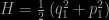
The solution of this system is well known: the general form is a sinusoidal motion and it is used in the description of all kinds of wave phenomena, swinging pendulums and so on.
The case Henon and Heiles looked at had two degrees of freedom, so that the Hamiltonian depends on q1, q2, p1 and p2:
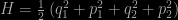
However, in this example, the two degrees of freedom are independent, meaning that there is uncoupled motion in the two directions. The amplitude of the oscillations is governed by the total energy of the system, which is a constant of the motion. Other than this, the type of behaviour displayed by this system is very rich, as exemplified by the various Lissajous figures shown in the diagram below. Note that all these figures are produced by the same type of dynamical system of equations: the different shapes are consequences of different initial conditions and different coefficients (which I set to unity in the form above).

If the oscillations in each direction have the same frequency then one can get an orbit which is a line or an ellipse. If the frequencies differ then the orbits can be much more complicated, but still pretty. Note that in all these cases the orbit is just a line, i.e. a one-dimensional part of the two-dimensional space drawn on the paper.
More generally, one can think of this system as a point moving in a four-dimensional phase space defined by the coordinates q1, q2, p1 and p2; taking slices through this space reveals qualitatively similar types of orbit for, say, p2 and q2 as for p1 and p2. The motion of the system is confined to a lower-dimensional part of the phase space rather than filling up all the available phase space. In this particular case, because each degree of freedom moves in only one of its two available dimensions, the system as a whole moves in a two-dimensional part of the four-dimensional space.
This all applies to the original, unperturbed system. Hénon and Heiles took this simple model and modified by adding a term to the Hamiltonian that was cubic rather than quadratic and which coupled the two degrees of freedom together. For those of you interested in the details their Hamiltonian was of the form

The first set of terms in the brackets is the unmodified form, describing a simple harmonic oscillator; the other two terms are new. The result of this simple alteration is really quite surprising. They found that, for low energies, the system continued to behave like two uncoupled oscillators; the orbits were smooth and well-behaved. This is not surprising because the cubic modifications are smaller than the original quadratic terms if the amplitude is small. For higher energies the motion becomes a bit more complicated, but the phase space behaviour is still characterized by continuous lines, as shown in the left hand part of the following figure.

However, at higher values of the energy (right), the cubic terms become more important, and something very striking happens. A two-dimensional slice through the phase space no longer shows the continuous curves that typify the original system, but a seemingly disorganized scattering of dots. It is not possible to discern any pattern in the phase space structure of this system: it appear to be random.
Nowadays we describe the transition from these two types of behaviour as being accompanied by the onset of chaos. It is important to note that this system is entirely deterministic, but it generates a phase space pattern that is quite different from what one would naively expect from the behaviour usually associated with classical Hamiltonian systems. To understand how this comes about it is perhaps helpful to think about predictability in classical systems. It is true that precise knowledge of the state of a system allows one to predict its state at some future time. For a single particle this means that precise knowledge of its position and momentum, and knowledge of the relevant H, will allow one to calculate the position and momentum at all future times.
But think a moment about what this means. What do we mean by precise knowledge of the particle’s position? How precise? How many decimal places? If one has to give the position exactly then that could require an infinite amount of information. Clearly we never have that much information. Everything we know about the physical world has to be coarse-grained to some extent, even if it is only limited by measurement error. Strict determinism in the form advocated by Laplace is clearly a fantasy. Determinism is not the same as predictability.
In “simple” Hamiltonian systems what happens is that two neighbouring phase-space paths separate from each other in a very controlled way as the system evolves. In fact the separation between paths usually grows proportionally to time. The coarse-graining with which the input conditions are specified thus leads to a similar level of coarse-graining in the output state. Effectively the system is predictable, since the uncertainty in the output is not much larger than in the input.
In the chaotic system things are very different. What happens here is that the non-linear interactions represented in the Hamiltonian play havoc with the initial coarse-graining. Phase-space orbits that start out close to each other separate extremely violently (typically exponentially) and in a way that varies from one part of the phase space to another. What happens then is that particle paths become hopelessly scrambled and the mapping between initial and final states becomes too complex to handle. What comes out the end is practically impossible to predict.


