Archive for the Bad Statistics Category

The Laws of Extremely Improbable Things

Posted in Bad Statistics, The Universe and Stuff with tags , , , , , , , , on June 9, 2011 by telescoper

After a couple of boozy nights in Copenhagen during the workshop which has just finished, I thought I’d take things easy this evening and make use of the free internet connection in my hotel to post a short item about something I talked about at the workshop here.

Actually I’ve been meaning to mention a nice bit of statistical theory called Extreme Value Theory on here for some time, because not so many people seem to be aware of it, but somehow I never got around to writing about it. People generally assume that statistical analysis of data revolves around “typical” quantities, such as averages or root-mean-square fluctuations (i.e. “standard” deviations). Sometimes, however, it’s not the typical points that are interesting, but those that appear to be drawn from the extreme tails of a probability distribution. This is particularly the case in planning for floods and other natural disasters, but this field also finds a number of interesting applications in astrophysics and cosmology. What should be the mass of the most massive cluster in my galaxy survey? How bright the brightest galaxy? How hot the hottest hotspot in the distribution of temperature fluctuations on the cosmic microwave background sky? And how cold the coldest? Sometimes just one anomalous event can be enormously useful in testing a theory.

I’m not going to go into the theory in any great depth here. Instead I’ll just give you a simple idea of how things work. First imagine you have a set of n observations labelled X_i. Assume that these are independent and identically distributed with a distribution function F(x), i.e.

\Pr(X_i\leq x)=F(x)

Now suppose you locate the largest value in the sample, X_{\rm max}. What is the distribution of this value? The answer is not F(x), but it is quite easy to work out because the probability that the largest value is less than or equal to, say, z is just the probability that each one is less than or equal to that value, i.e.

F_{\rm max}(z) = \Pr \left(X_{\rm max}\leq z\right)= \Pr \left(X_1\leq z, X_2\leq z\ldots, X_n\leq z\right)

Because the variables are independent and identically distributed, this means that

F_{\rm max} (z) = \left[ F(z) \right]^n

The probability density function associated with this is then just

f_{\rm max}(z) = n f(z) \left[ F(z) \right]^{n-1}

In a situation in which F(x) is known and in which the other assumptions apply, then this simple result offers the best way to proceed in analysing extreme values.

The mathematical interest in extreme values however derives from a paper in 1928 by Fisher \& Tippett which paved the way towards a general theory of extreme value distributions. I don’t want to go too much into details about that, but I will give a flavour by mentioning a historically important, perhaps surprising, and in any case rather illuminating example.

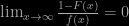
It turns out that for any distribution F(x) of exponential type, which means that

\lim_{x\rightarrow\infty} \frac{1-F(x)}{f(x)} = 0

then there is a stable asymptotic distribution of extreme values, as n \rightarrow \infty which is independent of the underlying distribution, F(x), and which has the form

G(z) = \exp \left(-\exp \left( -\frac{(z-a_n)}{b_n} \right)\right)

where a_n and b_n are location and scale parameters; this is called the Gumbel distribution. It’s not often you come across functions of the form e^{-e^{-y}}!

This result, and others, has established a robust and powerful framework for modelling extreme events. One of course has to be particularly careful if the variables involved are not independent (e.g. part of correlated sequences) or if there are not identically distributed (e.g. if the distribution is changing with time). One also has to be aware of the possibility that an extreme data point may simply be some sort of glitch (e.g. a cosmic ray hit on a pixel, to give an astronomical example). It should also be mentioned that the asymptotic theory is what it says on the tin – asymptotic. Some distributions of exponential type converge extremely slowly to the asymptotic form. A notable example is the Gaussian, which converges at the pathetically slow rate of \sqrt{\ln(n)}! This is why I advocate using the exact distribution resulting from a fully specified model whenever this is possible.

The pitfalls are dangerous and have no doubt led to numerous misapplications of this theory, but, done properly, it’s an approach that has enormous potential.

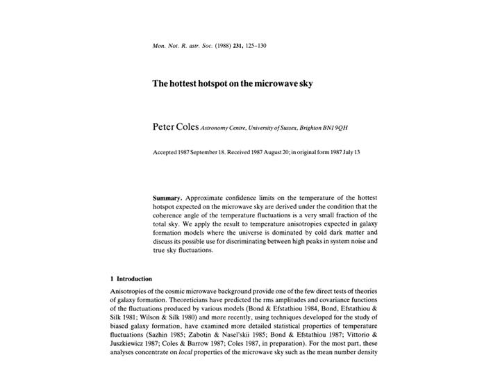
I’ve been interested in this branch of statistical theory for a long time, since I was introduced to it while I was a graduate student by a classic paper written by my supervisor. In fact I myself contributed to the classic old literature on this topic myself, with a paper on extreme temperature fluctuations in the cosmic microwave background way back in 1988..

Of course there weren’t any CMB maps back in 1988, and if I had thought more about it at the time I should have realised that since this was all done using Gaussian statistics, there was a 50% chance that the most interesting feature would actually be a negative rather than positive fluctuation. It turns out that twenty-odd years on, people are actually discussing an anomalous cold spot in the data from WMAP, proving that Murphy’s law applies to extreme events…

Guest Post – Bayesian Book Review

Posted in Bad Statistics, Books, Talks and Reviews with tags , , , on May 30, 2011 by telescoper

My regular commenter Anton circulated this book review by email yesterday and it stimulated quite a lot of reaction. I haven’t read the book myself, but I thought it would be fun to post his review on here to see whether it provokes similar responses. You can find the book on Amazon here (UK) or here ( USA). If you’re not completely au fait with Bayesian probability and the controversy around it, you might try reading one of my earlier posts about it, e.g. this one. I hope I can persuade some of the email commenters to upload their contributions through the box below!

-0-

The Theory That Would Not Die: How Bayes’ Rule Cracked the Enigma Code, Hunted Down Russian Submarines, and Emerged Triumphant from Two Centuries of Controversy

by Sharon Bertsch Mcgrayne

I found reading this book, which is a history of Bayes’ theorem written for the layman, to be deeply frustrating. The author does not really understand what probability IS – which is the key to all cogent writing on the subject. She never mentions the sum and product rules, or that Bayes’ theorem is an easy consequence of them. She notes, correctly, that Bayesian methods or something equivalent to them have been rediscovered advantageously again and again in an amazing variety of practical applications, and says that this is because they are pragmatically better than frequentist sampling theory – ie, she never asks the question: Why do they work better and what deeper rationale explains this? RT Cox is not mentioned. Ed Jaynes is mentioned only in passing as someone whose Bayesian fervour supposedly put people off.

The author is correct that computer applications have catalysed the Bayesian revolution, but in the pages on image processing and other general inverse problems (p218-21) she manages to miss the key work through the 1980s of Steve Gull and John Skilling, and you will not find “Maximum entropy” in the index. She does get the key role of Markov Chain Monte Carlo methods in computer implementation of Bayesian methods, however. But I can’t find Dave Mackay either, who deserves to be in the relevant section about modern applications.

On the other hand, as a historian of Bayesianism from Bayes himself to about 1960, she is full of superb anecdotes and information about
people who are to us merely names on the top of papers, or whose personalities are mentioned tantalisingly briefly in Jaynes’ writing.
For this material alone I recommend the book to Bayesians of our sort and am glad that I bought it.

Shooting at the Cosmic Circles

Posted in Astrohype, Bad Statistics, The Universe and Stuff with tags , , , , on May 11, 2011 by telescoper

Another brief update post of something that whizzed past while I was away and thought I’d mention now that I’m back.

Remember the (now infamous) paper by Gurzadyan and Penrose about evidence for the Conformal Cyclic Cosmology that I blogged about last year?

The original analysis was comprehensively dissected and refuted by a number of papers within a few days of its appearance – see here, here and here – only for Gurzadyan and Penrose to dig an even bigger hole for themselves with a nonsensical reply.

Undaunted, the dynamic duo of Gurzadyan and Penrose have produced yet another paper on the same subject which came out just as I was heading off on my hols.

There has subsequently been another riposte, by Eriksen and Wehus, although I suspect most cosmologists ceased to care about this whole story some time ago. Although it’s a pretty easy target, the Eriksen-Wehus reply does another comprehensive demolition job. The phrase “shooting fish in a barrel” sprang to my mind, but from facebook I learned that the equivalent idiomatic expression in Italian is sparare sulla Croce Rossa (i.e. shooting on the Red Cross). Perhaps we can add a brand new phrase for “taking aim at an easy target” – shooting at the cosmic circles!

I was struck, however, by the closing sentences of the abstract of Eriksen-Wehus reply:

Still, while this story is of little physical interest, it may have some important implications in terms of scienctific sociology: Looking back at the background papers leading up to the present series by Gurzadyan and Penrose, in particular one introducing the Kolmogorov statistic, we believe one can find evidence that a community based and open access referee process may be more efficient at rejecting incorrect results and claims than a traditional journal based approach.

I wholeheartedly agree. I’ve blogged already to the effect that academic journals are a waste of time and money and we’d be much better off with open access and vigorous internet scrutiny. It may be that this episode has just given us a glimpse of the future of scientific publishing.

Share/Bookmark

What Counts as Productivity?

Posted in Bad Statistics, Science Politics, The Universe and Stuff with tags , , , , on March 18, 2011 by telescoper

Apparently last year the United Kingdom Infra-Red Telescope (UKIRT) beat its own personal best for scientific productivity. In fact here’s a  graphic showing the number of publications resulting from UKIRT to make the point:

The plot also demonstrates that a large part of recent burst of productivity has been associated with UKIDSS (the UKIRT Infrared Deep Sky Survey) which a number of my colleagues are involved in. Excellent chaps. Great project. Lots of hard work done very well.  Take a bow, the UKIDSS team!

Now I hope I’ve made it clear that  I don’t in any way want to pour cold water on the achievements of UKIRT, and particularly not UKIDSS, but this does provide an example of how difficult it is to use bibliometric information in a meaningful way.

Take the UKIDSS papers used in the plot above. There are 226 of these listed by Steve Warren at Imperial College. But what is a “UKIDSS paper”? Steve states the criteria he adopted:

A paper is listed as a UKIDSS paper if it is already published in a journal (with one exception) and satisfies one of the following criteria:

1. It is one of the core papers describing the survey (e.g. calibration, archive, data releases). The DR2 paper is included, and is the only paper listed not published in a journal.
2. It includes science results that are derived in whole or in part from UKIDSS data directly accessed from the archive (analysis of data published in another paper does not count).
3. It contains science results from primary follow-up observations in a programme that is identifiable as a UKIDSS programme (e.g. The physical properties of four ~600K T dwarfs, presenting Spitzer spectra of cool brown dwarfs discovered with UKIDSS).
4. It includes a feasibility study of science that could be achieved using UKIDSS data (e.g. The possiblity of detection of ultracool dwarfs with the UKIRT Infrared Deep Sky Survey by Deacon and Hambly).

Papers are identified by a full-text search for the string ‘UKIDSS’, and then compared against the above criteria.

That all seems to me to by quite reasonable, and it’s certainly one way of defining what a UKIDSS paper is. According to that measure, UKIDSS scores 226.

The Warren measure does, however, include a number of papers that don’t directly use UKIDSS data, and many written by people who aren’t members of the UKIDSS consortium. Being picky you might say that such papers aren’t really original UKIDSS papers, but are more like second-generation spin-offs. So how could you count UKIDSS papers differently?

I just tried one alternative way, which is to use ADS to identify all refereed papers with “UKIDSS” in the title, assuming – possibly incorrectly – that all papers written by the UKIDSS consortium would have UKIDSS in the title. The number returned by this search was 38.

Now I’m not saying that this is more reasonable than the Warren measure. It’s just different, that’s all.  According to my criterion however UKIDSS measures 38 rather than 226. It sounds less impressive (if only because 38 is a smaller number than 226),  but what does it mean about UKIDSS productivity in absolute terms?

Not very much, I think is the answer.

Yet another way you might try to judge UKIDSS using bibliometric means is to look at its citation impact. After all, any fool can churn out dozens of papers that no-one ever reads. I know that for a fact. I am that fool.

But citation data also provide another way of doing what Steve Warren was trying to measure. Presumably the authors of any paper that uses UKIDSS data in any significant way would cite the main UKIDSS survey paper led by Andy Lawrence (Lawrence et al. 2007). According to ADS, the number of times this has been cited since publication is 359. That’s higher than the Warren measure (226), and much higher than the UKIDSS-in-the-title measure (38).

So there we are, three different measures, all in my opinion perfectly reasonable measures of, er,  something or other, but each giving a very different numerical value. I am not saying any  is misleading or that any is necessarily better than the others. My point is simply that it’s not easy to assign a numerical value to something that’s intrinsically difficult to define.

Unfortunately, it’s a point few people in government seem to be prepared to acknowledge.

Andy Lawrence is 57.


Share/Bookmark

A Census of the Ridiculous

Posted in Bad Statistics, History with tags , , , , on March 12, 2011 by telescoper

My form for the 2011 Census arrived yesterday. Apparently they were all posted out on Monday, so that’s 5 days in the post. Par for the course for the Royal Mail these days. I’m slightly surprised it arrived at all.

There’s a hefty £1000 fine for not completing the Census, so I suppose I’ll fill it in, despite my feeling that it’s both intrusive and unnecessary. What’s worse is that several of the questions are so badly designed that the information resulting will be useless.

For example, according to the census guide:

Very careful consideration is given to the questions included in the census. Questions must meet the needs of a substantial number of users in order that the census is acceptable to the public and yields good quality data. The questions are selected following several rounds of consultation with:

  • central and local government
  • academia
  • health authorities
  • the business community
  • groups representing ethnic minorities and others with special interests and concerns

Hang on. The “business community”? Why should they be consulted? What do they want with my personal information? I thought the census data was for planning public services!  On the other hand, when everything is privatised maybe all our personal data will be flogged off to the private sector anyway.

The 2011 Census is the first one to include a question on health. According to the saturation advertising about the census, this question will help plan new hospitals and distribute NHS funding. So what is the new question, the answer to which will provide such valuable data? Here it is, together with the possible responses:

13. How is your health in general?

  • Very good
  • Good
  • Fair
  • Bad
  • Very Bad

And that’s it for “health”. Does anyone actually believe such a vague question is  going to be of any use at all in planning NHS services? I certainly don’t.

And then there’s the famous question about religion.

20. What is your religion?

For a start I don’t think my religion or lack of it should be any concern to the government. To be fair, however, this question is marked as “voluntary” so respondents are allowed not to answer it without getting locked up in the Tower of London. But in any case it’s a leading question and should never have been included in the census in this form anyway. “Do you have a religion and, if so, what is it?” would have been much better.

I could go on, but I’ve got better things to do today.

I’ll just say this last thing about the Census. Most of it clearly has nothing whatever to do with planning public services. In fact the government already holds most of the information about your private circumstances the form demands. The Census is nothing more an opportunity for the government to cross-check tax, benefit or other records in the hope of finding inaccuracies. In other words, Big Brother is watching you.

And the cost of all this snooping? A whopping £500 million, more than double the cost of the 2001 Census, and all of it  at a time of huge cuts to public services. You have to laugh, don’t you?


Share/Bookmark

Bayes’ Razor

Posted in Bad Statistics, The Universe and Stuff with tags , , , , , , , , , on February 19, 2011 by telescoper

It’s been quite while since I posted a little piece about Bayesian probability. That one and the others that followed it (here and here) proved to be surprisingly popular so I’ve been planning to add a few more posts whenever I could find the time. Today I find myself in the office after spending the morning helping out with a very busy UCAS visit day, and it’s raining, so I thought I’d take the opportunity to write something before going home. I think I’ll do a short introduction to a topic I want to do a more technical treatment of in due course.

A particularly important feature of Bayesian reasoning is that it gives precise motivation to things that we are generally taught as rules of thumb. The most important of these is Ockham’s Razor. This famous principle of intellectual economy is variously presented in Latin as Pluralites non est ponenda sine necessitate or Entia non sunt multiplicanda praetor necessitatem. Either way, it means basically the same thing: the simplest theory which fits the data should be preferred.

William of Ockham, to whom this dictum is attributed, was an English Scholastic philosopher (probably) born at Ockham in Surrey in 1280. He joined the Franciscan order around 1300 and ended up studying theology in Oxford. He seems to have been an outspoken character, and was in fact summoned to Avignon in 1323 to account for his alleged heresies in front of the Pope, and was subsequently confined to a monastery from 1324 to 1328. He died in 1349.

In the framework of Bayesian inductive inference, it is possible to give precise reasons for adopting Ockham’s razor. To take a simple example, suppose we want to fit a curve to some data. In the presence of noise (or experimental error) which is inevitable, there is bound to be some sort of trade-off between goodness-of-fit and simplicity. If there is a lot of noise then a simple model is better: there is no point in trying to reproduce every bump and wiggle in the data with a new parameter or physical law because such features are likely to be features of the noise rather than the signal. On the other hand if there is very little noise, every feature in the data is real and your theory fails if it can’t explain it.

To go a bit further it is helpful to consider what happens when we generalize one theory by adding to it some extra parameters. Suppose we begin with a very simple theory, just involving one parameter p, but we fear it may not fit the data. We therefore add a couple more parameters, say q and r. These might be the coefficients of a polynomial fit, for example: the first model might be straight line (with fixed intercept), the second a cubic. We don’t know the appropriate numerical values for the parameters at the outset, so we must infer them by comparison with the available data.

Quantities such as p, q and r are usually called “floating” parameters; there are as many as a dozen of these in the standard Big Bang model, for example.

Obviously, having three degrees of freedom with which to describe the data should enable one to get a closer fit than is possible with just one. The greater flexibility within the general theory can be exploited to match the measurements more closely than the original. In other words, such a model can improve the likelihood, i.e. the probability  of the obtained data  arising (given the noise statistics – presumed known) if the signal is described by whatever model we have in mind.

But Bayes’ theorem tells us that there is a price to be paid for this flexibility, in that each new parameter has to have a prior probability assigned to it. This probability will generally be smeared out over a range of values where the experimental results (contained in the likelihood) subsequently show that the parameters don’t lie. Even if the extra parameters allow a better fit to the data, this dilution of the prior probability may result in the posterior probability being lower for the generalized theory than the simple one. The more parameters are involved, the bigger the space of prior possibilities for their values, and the harder it is for the improved likelihood to win out. Arbitrarily complicated theories are simply improbable. The best theory is the most probable one, i.e. the one for which the product of likelihood and prior is largest.

To give a more quantitative illustration of this consider a given model M which has a set of N floating parameters represented as a vector \underline\lambda = (\lambda_1,\ldots \lambda_N)=\lambda_i; in a sense each choice of parameters represents a different model or, more precisely, a member of the family of models labelled M.

Now assume we have some data D and can consequently form a likelihood function P(D|\underline{\lambda},M). In Bayesian reasoning we have to assign a prior probability P(\underline{\lambda}|M) to the parameters of the model which, if we’re being honest, we should do in advance of making any measurements!

The interesting thing to look at now is not the best-fitting choice of model parameters \underline{\lambda} but the extent to which the data support the model in general.  This is encoded in a sort of average of likelihood over the prior probability space:

P(D|M) = \int P(D|\underline{\lambda},M) P(\underline{\lambda}|M) d^{N}\underline{\lambda}.

This is just the normalizing constant K usually found in statements of Bayes’ theorem which, in this context, takes the form

P(\underline{\lambda}|DM) = K^{-1}P(\underline{\lambda}|M)P(D|\underline{\lambda},M).

In statistical mechanics things like K are usually called partition functions, but in this setting K is called the evidence, and it is used to form the so-called Bayes Factor, used in a technique known as Bayesian model selection of which more anon….

The  usefulness of the Bayesian evidence emerges when we ask the question whether our N  parameters are sufficient to get a reasonable fit to the data. Should we add another one to improve things a bit further? And why not another one after that? When should we stop?

The answer is that although adding an extra degree of freedom can increase the first term in the integral defining K (the likelihood), it also imposes a penalty in the second factor, the prior, because the more parameters the more smeared out the prior probability must be. If the improvement in fit is marginal and/or the data are noisy, then the second factor wins and the evidence for a model with N+1 parameters lower than that for the N-parameter version. Ockham’s razor has done its job.

This is a satisfying result that is in nice accord with common sense. But I think it goes much further than that. Many modern-day physicists are obsessed with the idea of a “Theory of Everything” (or TOE). Such a theory would entail the unification of all physical theories – all laws of Nature, if you like – into a single principle. An equally accurate description would then be available, in a single formula, of phenomena that are currently described by distinct theories with separate sets of parameters. Instead of textbooks on mechanics, quantum theory, gravity, electromagnetism, and so on, physics students would need just one book.

The physicist Stephen Hawking has described the quest for a TOE as like trying to read the Mind of God. I think that is silly. If a TOE is every constructed it will be the most economical available description of the Universe. Not the Mind of God.  Just the best way we have of saving paper.


Share/Bookmark

Deductivism and Irrationalism

Posted in Bad Statistics, The Universe and Stuff with tags , , , , , , , , , , , on December 11, 2010 by telescoper

Looking at my stats I find that my recent introductory post about Bayesian probability has proved surprisingly popular with readers, so I thought I’d follow it up with a brief discussion of some of the philosophical issues surrounding it.

It is ironic that the pioneers of probability theory, principally Laplace, unquestionably adopted a Bayesian rather than frequentist interpretation for his probabilities. Frequentism arose during the nineteenth century and held sway until recently. I recall giving a conference talk about Bayesian reasoning only to be heckled by the audience with comments about “new-fangled, trendy Bayesian methods”. Nothing could have been less apt. Probability theory pre-dates the rise of sampling theory and all the frequentist-inspired techniques that modern-day statisticians like to employ.

Most disturbing of all is the influence that frequentist and other non-Bayesian views of probability have had upon the development of a philosophy of science, which I believe has a strong element of inverse reasoning or inductivism in it. The argument about whether there is a role for this type of thought in science goes back at least as far as Roger Bacon who lived in the 13th Century. Much later the brilliant Scottish empiricist philosopher and enlightenment figure David Hume argued strongly against induction. Most modern anti-inductivists can be traced back to this source. Pierre Duhem has argued that theory and experiment never meet face-to-face because in reality there are hosts of auxiliary assumptions involved in making this comparison. This is nowadays called the Quine-Duhem thesis.

Actually, for a Bayesian this doesn’t pose a logical difficulty at all. All one has to do is set up prior probability distributions for the required parameters, calculate their posterior probabilities and then integrate over those that aren’t related to measurements. This is just an expanded version of the idea of marginalization, explained here.

Rudolf Carnap, a logical positivist, attempted to construct a complete theory of inductive reasoning which bears some relationship to Bayesian thought, but he failed to apply Bayes’ theorem in the correct way. Carnap distinguished between two types or probabilities – logical and factual. Bayesians don’t – and I don’t – think this is necessary. The Bayesian definition seems to me to be quite coherent on its own.

Other philosophers of science reject the notion that inductive reasoning has any epistemological value at all. This anti-inductivist stance, often somewhat misleadingly called deductivist (irrationalist would be a better description) is evident in the thinking of three of the most influential philosophers of science of the last century: Karl Popper, Thomas Kuhn and, most recently, Paul Feyerabend. Regardless of the ferocity of their arguments with each other, these have in common that at the core of their systems of thought likes the rejection of all forms of inductive reasoning. The line of thought that ended in this intellectual cul-de-sac began, as I stated above, with the work of the Scottish empiricist philosopher David Hume. For a thorough analysis of the anti-inductivists mentioned above and their obvious debt to Hume, see David Stove’s book Popper and After: Four Modern Irrationalists. I will just make a few inflammatory remarks here.

Karl Popper really began the modern era of science philosophy with his Logik der Forschung, which was published in 1934. There isn’t really much about (Bayesian) probability theory in this book, which is strange for a work which claims to be about the logic of science. Popper also managed to, on the one hand, accept probability theory (in its frequentist form), but on the other, to reject induction. I find it therefore very hard to make sense of his work at all. It is also clear that, at least outside Britain, Popper is not really taken seriously by many people as a philosopher. Inside Britain it is very different and I’m not at all sure I understand why. Nevertheless, in my experience, most working physicists seem to subscribe to some version of Popper’s basic philosophy.

Among the things Popper has claimed is that all observations are “theory-laden” and that “sense-data, untheoretical items of observation, simply do not exist”. I don’t think it is possible to defend this view, unless one asserts that numbers do not exist. Data are numbers. They can be incorporated in the form of propositions about parameters in any theoretical framework we like. It is of course true that the possibility space is theory-laden. It is a space of theories, after all. Theory does suggest what kinds of experiment should be done and what data is likely to be useful. But data can be used to update probabilities of anything.

Popper has also insisted that science is deductive rather than inductive. Part of this claim is just a semantic confusion. It is necessary at some point to deduce what the measurable consequences of a theory might be before one does any experiments, but that doesn’t mean the whole process of science is deductive. He does, however, reject the basic application of inductive reasoning in updating probabilities in the light of measured data; he asserts that no theory ever becomes more probable when evidence is found in its favour. Every scientific theory begins infinitely improbable, and is doomed to remain so.

Now there is a grain of truth in this, or can be if the space of possibilities is infinite. Standard methods for assigning priors often spread the unit total probability over an infinite space, leading to a prior probability which is formally zero. This is the problem of improper priors. But this is not a killer blow to Bayesianism. Even if the prior is not strictly normalizable, the posterior probability can be. In any case, given sufficient relevant data the cycle of experiment-measurement-update of probability assignment usually soon leaves the prior far behind. Data usually count in the end.

The idea by which Popper is best known is the dogma of falsification. According to this doctrine, a hypothesis is only said to be scientific if it is capable of being proved false. In real science certain “falsehood” and certain “truth” are almost never achieved. Theories are simply more probable or less probable than the alternatives on the market. The idea that experimental scientists struggle through their entire life simply to prove theorists wrong is a very strange one, although I definitely know some experimentalists who chase theories like lions chase gazelles. To a Bayesian, the right criterion is not falsifiability but testability, the ability of the theory to be rendered more or less probable using further data. Nevertheless, scientific theories generally do have untestable components. Any theory has its interpretation, which is the untestable baggage that we need to supply to make it comprehensible to us. But whatever can be tested can be scientific.

Popper’s work on the philosophical ideas that ultimately led to falsificationism began in Vienna, but the approach subsequently gained enormous popularity in western Europe. The American Thomas Kuhn later took up the anti-inductivist baton in his book The Structure of Scientific Revolutions. Kuhn is undoubtedly a first-rate historian of science and this book contains many perceptive analyses of episodes in the development of physics. His view of scientific progress is cyclic. It begins with a mass of confused observations and controversial theories, moves into a quiescent phase when one theory has triumphed over the others, and lapses into chaos again when the further testing exposes anomalies in the favoured theory. Kuhn adopted the word paradigm to describe the model that rules during the middle stage,

The history of science is littered with examples of this process, which is why so many scientists find Kuhn’s account in good accord with their experience. But there is a problem when attempts are made to fuse this historical observation into a philosophy based on anti-inductivism. Kuhn claims that we “have to relinquish the notion that changes of paradigm carry scientists ..closer and closer to the truth.” Einstein’s theory of relativity provides a closer fit to a wider range of observations than Newtonian mechanics, but in Kuhn’s view this success counts for nothing.

Paul Feyerabend has extended this anti-inductivist streak to its logical (though irrational) extreme. His approach has been dubbed “epistemological anarchism”, and it is clear that he believed that all theories are equally wrong. He is on record as stating that normal science is a fairytale, and that equal time and resources should be spent on “astrology, acupuncture and witchcraft”. He also categorised science alongside “religion, prostitution, and so on”. His thesis is basically that science is just one of many possible internally consistent views of the world, and that the choice between which of these views to adopt can only be made on socio-political grounds.

Feyerabend’s views could only have flourished in a society deeply disillusioned with science. Of course, many bad things have been done in science’s name, and many social institutions are deeply flawed. One can’t expect anything operated by people to run perfectly. It’s also quite reasonable to argue on ethical grounds which bits of science should be funded and which should not. But the bottom line is that science does have a firm methodological basis which distinguishes it from pseudo-science, the occult and new age silliness. Science is distinguished from other belief-systems by its rigorous application of inductive reasoning and its willingness to subject itself to experimental test. Not all science is done properly, of course, and bad science is as bad as anything.

The Bayesian interpretation of probability leads to a philosophy of science which is essentially epistemological rather than ontological. Probabilities are not “out there” in external reality, but in our minds, representing our imperfect knowledge and understanding. Scientific theories are not absolute truths. Our knowledge of reality is never certain, but we are able to reason consistently about which of our theories provides the best available description of what is known at any given time. If that description fails when more data are gathered, we move on, introducing new elements or abandoning the theory for an alternative. This process could go on forever. There may never be a final theory. But although the game might have no end, at least we know the rules….


Share/Bookmark

A Main Sequence for Galaxies?

Posted in Bad Statistics, The Universe and Stuff with tags , , , , , on December 2, 2010 by telescoper

Not for the first time in my life I find myself a bit of a laughing stock, after blowing my top during a seminar at Cardiff yesterday by retired Professor Mike Disney. In fact I got so angry that, much to the amusement of my colleagues, I stormed out. I don’t often lose my temper, and am not proud of having done so, but I reached a point when the red mist descended. What caused it was bad science and, in particular, bad statistics. It was all a big pity because what could have been an interesting discussion of an interesting result was ruined by too many unjustified assertions and too little attention to the underlying basis of the science. I still believe that no matter how interesting the results are, it’s  the method that really matters.

The interesting result that Mike Disney talked about emerges from a Principal Components Analysis (PCA) of the data relating to a sample of about 200 galaxies; it was actually published in Nature a couple of years ago; the arXiv version is here. It was the misleading way this was discussed in the seminar that got me so agitated so I’ll give my take on it now that I’ve calmed down to explain what I think is going on.

In fact, Principal Component Analysis is a very simple technique and shouldn’t really be controversial at all. It is a way of simplifying the representation of multivariate data by looking for the correlations present within it. To illustrate how it works, consider the following two-dimensional (i.e. bivariate) example I took from a nice tutorial on the method.

In this example the measured variables are Pressure and Temperature. When you plot them against each other you find they are correlated, i.e. the pressure tends to increase with temperature (or vice-versa). When you do a PCA of this type of dataset you first construct the covariance matrix (or, more precisely, its normalized form the correlation matrix). Such matrices are always symmetric and square (i.e. N×N, where N is the number of measurements involved at each point; in this case N=2) . What the PCA does is to determine the eigenvalues and eigenvectors of the correlation matrix.

The eigenvectors for the example above are shown in the diagram – they are basically the major and minor axes of an ellipse drawn to fit the scatter plot; these two eigenvectors (and their associated eigenvalues) define the principal components as linear combinations of the original variables. Notice that along one principal direction (v1) there is much more variation than the other (v2). This means that most of the variance in the data set is along the direction indicated by the vector v1, and relatively little in the orthogonal direction v2; the eigenvalue for the first vector is consequently larger than that for the second.

The upshot of this is that the description of this (very simple) dataset can be compressed by using the first principal component rather than the original variables, i.e. by switching from the original two variables (pressure and temperature) to one variable (v1) we have compressed our description without losing much information (only the little bit that is involved in the scatter in the v2 direction.

In the more general case of N observables there will be N principal components, corresponding to vectors in an N-dimensional space, but nothing changes qualitatively. What the PCA does is to rank the eigenvectors according to their eigenvalue (i.e. the variance associated with the direction of the eigenvector). The first principal component is the one with the largest variance, and so on down the ordered list.

Where PCA is useful with large data sets is when the variance associated with the first (or first few) principal components is very much larger than the rest. In that case one can dispense with the N variables and just use one or two.

In the cases discussed by Professor Disney yesterday the data involved six measurable parameters of each galaxy: (1) a dynamical mass estimate; (2) the mass inferred from HI emission (21cm); (3) the total luminosity; (4) radius; (5) a measure of the central concentration of the galaxy; and (6) a measure of its colour. The PCA analysis of these data reveals that about 80% of the variance in the data set is associated with the first principal component, so there is clearly a significant correlation present in the data although, to be honest, I have seen many PCA analyses with much stronger concentrations of variance in the first eigenvector so it doesn’t strike me as being particularly strong.

However, thinking as a physicist rather than a statistician there is clearly something very interesting going on. From a theoretical point of view one would imagine that the properties of an individual galaxy might be controlled by as many as six independent parameters including mass, angular momentum, baryon fraction, age and size, as well as by the accidents of its recent haphazard merger history.

Disney et al. argue that for gaseous galaxies to appear as a one-parameter set, as observed here, the theory of galaxy formation and evolution must supply at least five independent constraint equations in order to collapse everything into a single parameter.

This is all vaguely reminiscent of the Hertzsprung-Russell diagram, or at least the main sequence thereof:


You can see here that there’s a correlation between temperature and luminosity which constrains this particular bivariate data set to lie along a (nearly) one-dimensional track in the diagram. In fact these properties correlate with each other because there is a single parameter model relating all properties of main sequence stars to their mass. In other words, once you fix the mass of a main sequence star, it has a fixed  luminosity, temperature, and radius (apart from variations caused by age, metallicity, etc). Of course the problem is that masses of stars are difficult to determine so this parameter is largely hidden from the observer. What is really happening is that luminosity and temperature correlate with each other, because they both depend on the  hidden parameter mass.

I don’t think that the PCA result disproves the current theory of hierarchical galaxy formation (which is what Disney claims) but it will definitely be a challenge for theorists to provide a satisfactory explanation of the result! My own guess for the physical parameter that accounts for most of the variation in this data set is the mass of the dark halo within which the galaxy is embedded. In other words, it might really be just like the Hertzsprung-Russell diagram…

But back to my argument with Mike Disney. I asked what is the first principal component of the galaxy data, i.e. what does the principal eigenvector look like? He refused to answer, saying that it was impossible to tell. Of course it isn’t, as the PCA method actually requires it to be determined. Further questioning seemed to reveal a basic misunderstanding of the whole idea of PCA which made the assertion that all of modern cosmology would need to be revised somewhat difficult to swallow.  At that point of deadlock, I got very angry and stormed out.

I realise that behind the confusion was a reasonable point. The first principal component is well-defined, i.e. v1 is completely well defined in the first figure. However, along the line defined by that vector, P and T are proportional to each other so in a sense only one of them is needed to specify a position along this line. But you can’t say on the basis of this analysis alone that the fundamental variable is either pressure or temperature; they might be correlated through a third quantity you don’t know about.

Anyway, as a postscript I’ll say I did go and apologize to Mike Disney afterwards for losing my rag. He was very forgiving, although I probably now have a reputation for being a grumpy old bastard. Which I suppose I am. He also said one other thing,  that he didn’t mind me getting angry because it showed I cared about the truth. Which I suppose I do.


Share/Bookmark

Doubts about the Evidence for Penrose’s Cyclic Universe

Posted in Bad Statistics, Cosmic Anomalies, The Universe and Stuff with tags , , , , , , on November 28, 2010 by telescoper

A strange paper by Gurzadyan and Penrose hit the Arxiv a week or so ago. It seems to have generated quite a lot of reaction in the blogosphere and has now made it onto the BBC News, so I think it merits a comment.

The authors claim to have found evidence that supports Roger Penrose‘s conformal cyclic cosmology in the form of a series of (concentric) rings of unexpectedly low variance in the pattern of fluctuations in the cosmic microwave background seen by the Wilkinson Microwave Anisotropy Probe (WMAP). There’s no doubt that a real discovery of such signals in the WMAP data would point towards something radically different from the standard Big Bang cosmology.

I haven’t tried to reproduce Gurzadyan & Penrose’s result in detail, as I haven’t had time to look at it, and I’m not going to rule it out without doing a careful analysis myself. However, what I will say here is that I think you should take the statistical part of their analysis with a huge pinch of salt.

Here’s why.

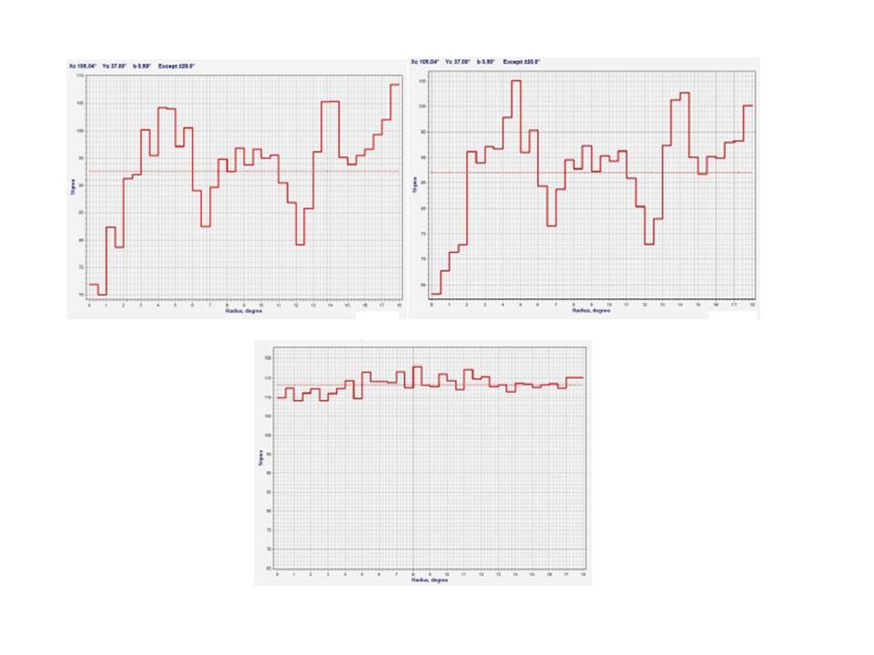
The authors report a hugely significant detection of their effect (they quote a “6-σ” result; in other words, the expected feature is expected to arise in the standard cosmological model with a probability of less than 10-7. The type of signal can be seen in their Figure 2, which I reproduce here:

Sorry they’re hard to read, but these show the variance measured on concentric rings (y-axis) of varying radius (x-axis) as seen in the WMAP W (94 Ghz) and V (54 Ghz) frequency channels (top two panels) compared with what is seen in a simulation with purely Gaussian fluctuations generated within the framework of the standard cosmological model (lower panel). The contrast looks superficially impressive, but there’s much less to it than meets the eye.

For a start, the separate WMAP W and V channels are not the same as the cosmic microwave background. There is a great deal of galactic foreground that has to be cleaned out of these maps before the pristine primordial radiation can be isolated. The fact similar patterns can be found in the BOOMERANG data by no means rules out a foreground contribution as a common explanation of anomalous variance. The authors have excluded the region at low galactic latitude (|b|<20°) in order to avoid the most heavily contaminated parts of the sky, but this is by no means guaranteed to eliminate foreground contributions entirely. Here is the all-sky WMAP W-band map for example:

Moreover, these maps also contain considerable systematic effects arising from the scanning strategy of the WMAP satellite. The most obvious of these is that the signal-to-noise varies across the sky, but there are others, such as the finite size of the beam of the WMAP telescope.

Neither galactic foregrounds nor correlated noise are present in the Gaussian simulation shown in the lower panel, and the authors do not say what kind of beam smoothing is used either. The comparison of WMAP single-channel data with simple Gaussian simulations is consequently deeply flawed and the significance level quoted for the result is certainly meaningless.

Having not looked looked at this in detail myself I’m not going to say that the authors’ conclusions are necessarily false, but I would be very surprised if an effect this large was real given the strenuous efforts so many people have made to probe the detailed statistics of the WMAP data; see, e.g., various items in my blog category on cosmic anomalies. Cosmologists have been wrong before, of course, but then so have even eminent physicists like Roger Penrose…

Another point that I’m not sure about at all is even if the rings of low variance are real – which I doubt – do they really provide evidence of a cyclic universe? It doesn’t seem obvious to me that the model Penrose advocates would actually produce a CMB sky that had such properties anyway.

Above all, I stress that this paper has not been subjected to proper peer review. If I were the referee I’d demand a much higher level of rigour in the analysis before I would allow it to be published in a scientific journal. Until the analysis is done satisfactorily, I suggest that serious students of cosmology shouldn’t get too excited by this result.

It occurs to me that other cosmologists out there might have looked at this result in more detail than I have had time to. If so, please feel free to add your comments in the box…

IMPORTANT UPDATE: 7th December. Two papers have now appeared on the arXiv (here and here) which refute the Gurzadyan-Penrose claim. Apparently, the data behave as Gurzadyan and Penrose claim, but so do proper simulations. In otherwords, it’s the bottom panel of the figure that’s wrong.

ANOTHER UPDATE: 8th December. Gurzadyan and Penrose have responded with a two-page paper which makes so little sense I had better not comment at all.


Share/Bookmark

Bayes and his Theorem

Posted in Bad Statistics with tags , , , , , , on November 23, 2010 by telescoper

My earlier post on Bayesian probability seems to have generated quite a lot of readers, so this lunchtime I thought I’d add a little bit of background. The previous discussion started from the result

P(B|AC) = K^{-1}P(B|C)P(A|BC) = K^{-1} P(AB|C)

where

K=P(A|C).

Although this is called Bayes’ theorem, the general form of it as stated here was actually first written down, not by Bayes but by Laplace. What Bayes’ did was derive the special case of this formula for “inverting” the binomial distribution. This distribution gives the probability of x successes in n independent “trials” each having the same probability of success, p; each “trial” has only two possible outcomes (“success” or “failure”). Trials like this are usually called Bernoulli trials, after Daniel Bernoulli. If we ask the question “what is the probability of exactly x successes from the possible n?”, the answer is given by the binomial distribution:

P_n(x|n,p)= C(n,x) p^x (1-p)^{n-x}

where

C(n,x)= n!/x!(n-x)!

is the number of distinct combinations of x objects that can be drawn from a pool of n.

You can probably see immediately how this arises. The probability of x consecutive successes is p multiplied by itself x times, or px. The probability of (n-x) successive failures is similarly (1-p)n-x. The last two terms basically therefore tell us the probability that we have exactly x successes (since there must be n-x failures). The combinatorial factor in front takes account of the fact that the ordering of successes and failures doesn’t matter.

The binomial distribution applies, for example, to repeated tosses of a coin, in which case p is taken to be 0.5 for a fair coin. A biased coin might have a different value of p, but as long as the tosses are independent the formula still applies. The binomial distribution also applies to problems involving drawing balls from urns: it works exactly if the balls are replaced in the urn after each draw, but it also applies approximately without replacement, as long as the number of draws is much smaller than the number of balls in the urn. I leave it as an exercise to calculate the expectation value of the binomial distribution, but the result is not surprising: E(X)=np. If you toss a fair coin ten times the expectation value for the number of heads is 10 times 0.5, which is five. No surprise there. After another bit of maths, the variance of the distribution can also be found. It is np(1-p).

So this gives us the probability of x given a fixed value of p. Bayes was interested in the inverse of this result, the probability of p given x. In other words, Bayes was interested in the answer to the question “If I perform n independent trials and get x successes, what is the probability distribution of p?”. This is a classic example of inverse reasoning. He got the correct answer, eventually, but by very convoluted reasoning. In my opinion it is quite difficult to justify the name Bayes’ theorem based on what he actually did, although Laplace did specifically acknowledge this contribution when he derived the general result later, which is no doubt why the theorem is always named in Bayes’ honour.

This is not the only example in science where the wrong person’s name is attached to a result or discovery. In fact, it is almost a law of Nature that any theorem that has a name has the wrong name. I propose that this observation should henceforth be known as Coles’ Law.

So who was the mysterious mathematician behind this result? Thomas Bayes was born in 1702, son of Joshua Bayes, who was a Fellow of the Royal Society (FRS) and one of the very first nonconformist ministers to be ordained in England. Thomas was himself ordained and for a while worked with his father in the Presbyterian Meeting House in Leather Lane, near Holborn in London. In 1720 he was a minister in Tunbridge Wells, in Kent. He retired from the church in 1752 and died in 1761. Thomas Bayes didn’t publish a single paper on mathematics in his own name during his lifetime but despite this was elected a Fellow of the Royal Society (FRS) in 1742. Presumably he had Friends of the Right Sort. He did however write a paper on fluxions in 1736, which was published anonymously. This was probably the grounds on which he was elected an FRS.

The paper containing the theorem that now bears his name was published posthumously in the Philosophical Transactions of the Royal Society of London in 1764.

P.S. I understand that the authenticity of the picture is open to question. Whoever it actually is, he looks  to me a bit like Laurence Olivier…


Share/Bookmark