Archive for the Bad Statistics Category

The Doomsday Argument

Posted in Bad Statistics, The Universe and Stuff with tags , , , , , on April 29, 2009 by telescoper

I don’t mind admitting that as I get older I get more and  more pessimistic about the prospects for humankind’s survival into the distant future.

Unless there are major changes in the way this planet is governed, our planet may become barren and uninhabitable through war or environmental catastrophe. But I do think the future is in our hands, and disaster is, at least in principle, avoidable. In this respect I have to distance myself from a very strange argument that has been circulating among philosophers and physicists for a number of years. It is called Doomsday argument, and it even has a sizeable wikipedia entry, to which I refer you for more details and variations on the basic theme. As far as I am aware, it was first introduced by the mathematical physicist Brandon Carter and subsequently developed and expanded by the philosopher John Leslie (not to be confused with the TV presenter of the same name). It also re-appeared in slightly different guise through a paper in the serious scientific journal Nature by the eminent physicist Richard Gott. Evidently, for some reason, some serious people take it very seriously indeed.

The Doomsday argument uses the language of probability theory, but it is such a strange argument that I think the best way to explain it is to begin with a more straightforward problem of the same type.

 Imagine you are a visitor in an unfamiliar, but very populous, city. For the sake of argument let’s assume that it is in China. You know that this city is patrolled by traffic wardens, each of whom carries a number on their uniform.  These numbers run consecutively from 1 (smallest) to T (largest) but you don’t know what T is, i.e. how many wardens there are in total. You step out of your hotel and discover traffic warden number 347 sticking a ticket on your car. What is your best estimate of T, the total number of wardens in the city?

 I gave a short lunchtime talk about this when I was working at Queen Mary College, in the University of London. Every Friday, over beer and sandwiches, a member of staff or research student would give an informal presentation about their research, or something related to it. I decided to give a talk about bizarre applications of probability in cosmology, and this problem was intended to be my warm-up. I was amazed at the answers I got to this simple question. The majority of the audience denied that one could make any inference at all about T based on a single observation like this, other than that it  must be at least 347.

 Actually, a single observation like this can lead to a useful inference about T, using Bayes’ theorem. Suppose we have really no idea at all about T before making our observation; we can then adopt a uniform prior probability. Of course there must be an upper limit on T. There can’t be more traffic wardens than there are people, for example. Although China has a large population, the prior probability of there being, say, a billion traffic wardens in a single city must surely be zero. But let us take the prior to be effectively constant. Suppose the actual number of the warden we observe is t. Now we have to assume that we have an equal chance of coming across any one of the T traffic wardens outside our hotel. Each value of t (from 1 to T) is therefore equally likely. I think this is the reason that my astronomers’ lunch audience thought there was no information to be gleaned from an observation of any particular value, i.e. t=347.

 Let us simplify this argument further by allowing two alternative “models” for the frequency of Chinese traffic wardens. One has T=1000, and the other (just to be silly) has T=1,000,000. If I find number 347, which of these two alternatives do you think is more likely? Think about the kind of numbers that occupy the range from 1 to T. In the first case, most of the numbers have 3 digits. In the second, most of them have 6. If there were a million traffic wardens in the city, it is quite unlikely you would find a random individual with a number as small as 347. If there were only 1000, then 347 is just a typical number. There are strong grounds for favouring the first model over the second, simply based on the number actually observed. To put it another way, we would be surprised to encounter number 347 if T were actually a million. We would not be surprised if T were 1000.

 One can extend this argument to the entire range of possible values of T, and ask a more general question: if I observe traffic warden number t what is the probability I assign to each value of T? The answer is found using Bayes’ theorem. The prior, as I assumed above, is uniform. The likelihood is the probability of the observation given the model. If I assume a value of T, the probability P(t|T) of each value of t (up to and including T) is just 1/T (since each of the wardens is equally likely to be encountered). Bayes’ theorem can then be used to construct a posterior probability of P(T|t). Without going through all the nuts and bolts, I hope you can see that this probability will tail off for large T. Our observation of a (relatively) small value for t should lead us to suspect that T is itself (relatively) small. Indeed it’s a reasonable “best guess” that T=2t. This makes intuitive sense because the observed value of t then lies right in the middle of its range of possibilities.

 Before going on, it is worth mentioning one other point about this kind of inference: that it is not at all powerful. Note that the likelihood just varies as 1/T. That of course means that small values are favoured over large ones. But note that this probability is uniform in logarithmic terms. So although T=1000 is more probable than T=1,000,000,  the range between 1000 and 10,000 is roughly as likely as the range between 1,000,000 and 10,000,0000, assuming there is no prior information. So although it tells us something, it doesn’t actually tell us very much. Just like any probabilistic inference, there’s a chance that it is wrong, perhaps very wrong.

 What does all this have to do with Doomsday? Instead of traffic wardens, we want to estimate N, the number of humans that will ever be born, Following the same logic as in the example above, I assume that I am a “randomly” chosen individual drawn from the sequence of all humans to be born, in past present and future. For the sake of argument, assume I number n in this sequence. The logic I explained above should lead me to conclude that the total number N is not much larger than my number, n. For the sake of argument, assume that I am the one-billionth human to be born, i.e. n=1,000,000,0000.  There should not be many more than a few billion humans ever to be born. At the rate of current population growth, this means that not many more generations of humans remain to be born. Doomsday is nigh.

 Richard Gott’s version of this argument is logically similar, but is based on timescales rather than numbers. If whatever thing we are considering begins at some time tbegin and ends at a time tend and if we observe it at a “random” time between these two limits, then our best estimate for its future duration is of order how long it has lasted up until now. Gott gives the example of Stonehenge[1], which was built about 4,000 years ago: we should expect it to last a few thousand years into the future. Actually, Stonehenge is a highly dubious . It hasn’t really survived 4,000 years. It is a ruin, and nobody knows its original form or function. However, the argument goes that if we come across a building put up about twenty years ago, presumably we should think it will come down again (whether by accident or design) in about twenty years time. If I happen to walk past a building just as it is being finished, presumably I should hang around and watch its imminent collapse….

But I’m being facetious.

Following this chain of thought, we would argue that, since humanity has been around a few hundred thousand years, it is expected to last a few hundred thousand years more. Doomsday is not quite as imminent as previously, but in any case humankind is not expected to survive sufficiently long to, say, colonize the Galaxy.

 You may reject this type of argument on the grounds that you do not accept my logic in the case of the traffic wardens. If so, I think you are wrong. I would say that if you accept all the assumptions entering into the Doomsday argument then it is an equally valid example of inductive inference. The real issue is whether it is reasonable to apply this argument at all in this particular case. There are a number of related examples that should lead one to suspect that something fishy is going on. Usually the problem can be traced back to the glib assumption that something is “random” when or it is not clearly stated what that is supposed to mean.

 There are around sixty million British people on this planet, of whom I am one. In contrast there are 3 billion Chinese. If I follow the same kind of logic as in the examples I gave above, I should be very perplexed by the fact that I am not Chinese. After all, the odds are 50: 1 against me being British, aren’t they?

 Of course, I am not at all surprised by the observation of my non-Chineseness. My upbringing gives me access to a great deal of information about my own ancestry, as well as the geographical and political structure of the planet. This data convinces me that I am not a “random” member of the human race. My self-knowledge is conditioning information and it leads to such a strong prior knowledge about my status that the weak inference I described above is irrelevant. Even if there were a million million Chinese and only a hundred British, I have no grounds to be surprised at my own nationality given what else I know about how I got to be here.

 This kind of conditioning information can be applied to history, as well as geography. Each individual is generated by its parents. Its parents were generated by their parents, and so on. The genetic trail of these reproductive events connects us to our primitive ancestors in a continuous chain. A well-informed alien geneticist could look at my DNA and categorize me as an “early human”. I simply could not be born later in the story of humankind, even if it does turn out to continue for millennia. Everything about me – my genes, my physiognomy, my outlook, and even the fact that I bothering to spend time discussing this so-called paradox – is contingent on my specific place in human history. Future generations will know so much more about the universe and the risks to their survival that they won’t even discuss this simple argument. Perhaps we just happen to be living at the only epoch in human history in which we know enough about the Universe for the Doomsday argument to make some kind of sense, but too little to resolve it.

 To see this in a slightly different light, think again about Gott’s timescale argument. The other day I met an old friend from school days. It was a chance encounter, and I hadn’t seen the person for over 25 years. In that time he had married, and when I met him he was accompanied by a baby daughter called Mary. If we were to take Gott’s argument seriously, this was a random encounter with an entity (Mary) that had existed for less than a year. Should I infer that this entity should probably only endure another year or so? I think not. Again, bare numerological inference is rendered completely irrelevant by the conditioning information I have. I know something about babies. When I see one I realise that it is an individual at the start of its life, and I assume that it has a good chance of surviving into adulthood. Human civilization is a baby civilization. Like any youngster, it has dangers facing it. But is not doomed by the mere fact that it is young,

 John Leslie has developed many different variants of the basic Doomsday argument, and I don’t have the time to discuss them all here. There is one particularly bizarre version, however, that I think merits a final word or two because is raises an interesting red herring. It’s called the “Shooting Room”.

 Consider the following model for human existence. Souls are called into existence in groups representing each generation. The first generation has ten souls. The next has a hundred, the next after that a thousand, and so on. Each generation is led into a room, at the front of which is a pair of dice. The dice are rolled. If the score is double-six then everyone in the room is shot and it’s the end of humanity. If any other score is shown, everyone survives and is led out of the Shooting Room to be replaced by the next generation, which is ten times larger. The dice are rolled again, with the same rules. You find yourself called into existence and are led into the room along with the rest of your generation. What should you think is going to happen?

 Leslie’s argument is the following. Each generation not only has more members than the previous one, but also contains more souls than have ever existed to that point. For example, the third generation has 1000 souls; the previous two had 10 and 100 respectively, i.e. 110 altogether. Roughly 90% of all humanity lives in the last generation. Whenever the last generation happens, there bound to be more people in that generation than in all generations up to that point. When you are called into existence you should therefore expect to be in the last generation. You should consequently expect that the dice will show double six and the celestial firing squad will take aim. On the other hand, if you think the dice are fair then each throw is independent of the previous one and a throw of double-six should have a probability of just one in thirty-six. On this basis, you should expect to survive. The odds are against the fatal score.

 This apparent paradox seems to suggest that it matters a great deal whether the future is predetermined (your presence in the last generation requires the double-six to fall) or “random” (in which case there is the usual probability of a double-six). Leslie argues that if everything is pre-determined then we’re doomed. If there’s some indeterminism then we might survive. This isn’t really a paradox at all, simply an illustration of the fact that assuming different models gives rise to different probability assignments.

 While I am on the subject of the Shooting Room, it is worth drawing a parallel with another classic puzzle of probability theory, the St Petersburg Paradox. This is an old chestnut to do with a purported winning strategy for Roulette. It was first proposed by Nicolas Bernoulli but famously discussed at greatest length by Daniel Bernoulli in the pages of Transactions of the St Petersburg Academy, hence the name.  It works just as well for the case of a simple toss of a coin as for Roulette as in the latter game it involves betting only on red or black rather than on individual numbers.

 Imagine you decide to bet such that you win by throwing heads. Your original stake is £1. If you win, the bank pays you at even money (i.e. you get your stake back plus another £1). If you lose, i.e. get tails, your strategy is to play again but bet double. If you win this time you get £4 back but have bet £2+£1=£3 up to that point. If you lose again you bet £8. If you win this time, you get £16 back but have paid in £8+£4+£2+£1=£15 to that point. Clearly, if you carry on the strategy of doubling your previous stake each time you lose, when you do eventually win you will be ahead by £1. It’s a guaranteed winner. Isn’t it?

 The answer is yes, as long as you can guarantee that the number of losses you will suffer is finite. But in tosses of a fair coin there is no limit to the number of tails you can throw before getting a head. To get the correct probability of winning you have to allow for all possibilities. So what is your expected stake to win this £1? The answer is the root of the paradox. The probability that you win straight off is ½ (you need to throw a head), and your stake is £1 in this case so the contribution to the expectation is £0.50. The probability that you win on the second go is ¼ (you must lose the first time and win the second so it is ½ times ½) and your stake this time is £2 so this contributes the same £0.50 to the expectation. A moment’s thought tells you that each throw contributes the same amount, £0.50, to the expected stake. We have to add this up over all possibilities, and there are an infinite number of them. The result of summing them all up is therefore infinite. If you don’t believe this just think about how quickly your stake grows after only a few losses: £1, £2, £4, £8, £16, £32, £64, £128, £256, £512, £1024, etc. After only ten losses you are staking over a thousand pounds just to get your pound back. Sure, you can win £1 this way, but you need to expect to stake an infinite amount to guarantee doing so. It is not a very good way to get rich.

 The relationship of all this to the Shooting Room is that it is shows it is dangerous to pre-suppose a finite value for a number which in principle could be infinite. If the number of souls that could be called into existence is allowed to be infinite, then any individual as no chance at all of being called into existence in any generation!

 Amusing as they are, the thing that makes me most uncomfortable about these Doomsday arguments is that they attempt to determine a probability of an event without any reference to underlying mechanism. For me, a valid argument about Doomsday would have to involve a particular physical cause for the extinction of humanity (e.g. asteroid impact, climate change, nuclear war, etc). Given this physical mechanism one should construct a model within which one can estimate probabilities for the model parameters (such as the rate of occurrence of catastrophic asteroid impacts). Only then can one make a valid inference based on relevant observations and their associated likelihoods. Such calculations may indeed lead to alarming or depressing results. I fear that the greatest risk to our future survival is not from asteroid impact or global warming, where the chances can be estimated with reasonable precision, but self-destructive violence carried out by humans themselves. Science has no way of being able to predict what atrocities people are capable of so we can’t make any reliable estimate of the probability we will self-destruct. But the absence of any specific mechanism in the versions of the Doomsday argument I have discussed robs them of any scientific credibility at all.

There are better grounds for worrying about the future than mere numerology.

The First Digit Phenomenon

Posted in Bad Statistics, The Universe and Stuff with tags , , on March 11, 2009 by telescoper

I thought it would be fun to put up this quirky example of how sometimes things that really ought to be random turn out not to be. It’s also an excuse to mention a strange connection between astronomy and statistics.

The astronomer Simon Newcomb (right) was born in 1835 in Nova Scotia picture2(Canada). He had no real formal education at all, but since there wasn’t much else to do in Nova Scotia, he taught himself mathematics and astronomy and became very adept at performing astronomical calculations with great diligence. He began work in a lowly position at the US Nautical Almanac Office in 1857, and by 1877 he was director. He became was professor of Mathematics and Astronomy and Johns Hopkins University from 1884 until 1893 and was made the first ever president of the American Astronomical Society in 1899; he died in 1909.
Newcomb was performing lengthy numerical calculations in an era long before the invention of the pocket calculator or desktop computer. In those days many such calculations, including virtually anything involving multiplication, had to be done using logarithms. The logarithm (to the base ten) of a number x is defined to be the number a such that x=10a. To multiply two numbers whose logarithms are a and b respectively involves simply adding the logarithms: 10a times 10b=10(a+b), which helps a lot because adding is a lot easier than multiplying if you have no calculator. The initial logarithms are simply looked up in a table; to find the answer you use different tables to find the “inverse” logarithm.

Newcomb was a heavy user of his book of mathematical tables for this type of calculation, and it became very grubby and worn. But he also noticed that the first pages of the logarithms seemed to have been used much more than the others. This puzzled him greatly. Logarithm tables are presented in order of the first digit of the number required: the first pages therefore contain logarithms for numbers beginning with the digit 1. Newcomb used the tables for a vast range of different calculations of different things. He expected the first digits of numbers that he had to look up to just be as likely to be anything. Shouldn’t they be randomly distributed? Shouldn’t all the pages be equally used?

Once raised, this puzzle faded away until it was re-discovered in 1938 and acquired the name of Benford’s law, or the first digit phenomenon. In virtually any list you can think of – street addresses, city populations, lengths of rivers, and so on – there are more entries beginning with the digit “1” than any other digit.

To give another example, although I admit this one is much harder to explain, in the American Physical Society’s list of fundamental constants, or at least the last version I happened to look at, no less than 40% begin with the digit 1. If you’ve been writing physics examination papers recently like I have, you will notice a similar behaviour. Out of the 16 physical constants listed in the rubric of a physics examination paper lying on my desk right now, 6 begin with the digit 1.

So what is going on?

There is a (relatively) simple answer, and a more complicated one. I’ll take the simple one first.

Consider street numbers in an address book as an example. Suppose Any street will be numbered from 1 to N. It doesn’t really matter what N is as long as it is finite (and nobody has ever built an infinitely long street). Now think about the first digits of the addresses. There are 9 possibilities, because we never start an address with 0. On the face of it, we might expect a fraction 1/9 (approximately 11%) of the addresses will start with 1. Suppose N is 200. What fraction actually starts with 1? The answer is more than 50%. Everything from 100 upwards, plus 1, and 11 to 19. Very few start with 9: only 9 itself, and 90-99 inclusive. If N is 300 then there are still more beginning with 1 than any other digit, and there are no more that start with 9. One only gets close to an equal fraction of each starting number if the value of N is an exact power of 10, e.g. 1000.

Now you can see why pulling numbers out of an address book leads to a distribution of first digits that is not at all uniform. As long as the numbers are being drawn from a collection of streets each of whom has a finite upper limit, then the result is bound to be biased towards low starting digits. Only if every street contained an exact power of ten addresses would the result be uniform. Every other possibility favours 1 at the start.

The more complicated version involves a scaling argument and is a more suitable explanation for the appearance of this phenomenon in measured physical quantities. Lengths, heights and weights of things are usually measured with respect to some reference quantity. In the absence of any other information, one might imagine that the distribution of whatever is being measured possesses some sort of invariance or symmetry with respect to the scale being chosen. In this case the prior distribution p(x) can be taken to have the so-called Jeffreys form, which is uniform in the logarithm, i.e. p(x) is proportional to 1/x. There obviously must be a cut-off at some point as this can’t be allowed to go on forever as it doesn’t converge for large x, but this doesn’t really matter for the sake of this argument. We can suppose anyway that there are many powers of ten involved before this upper limit is reached.

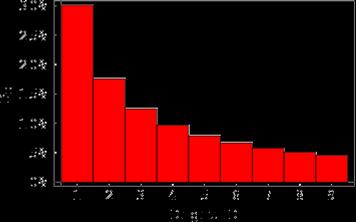
In this case the probability that the first digit is D is just given by the ratio of two terms: In the numerator we have the integral between D and D+1 of p(x) (that’s a measure of how much of the distribution represents numbers starting with the digit D) and on the denominator we have the integral between 1 and 10 of p(x) (the overall measure). The result, if we take p(x) to be proportional to 1/x, is just log (1+1/D).

picture1

The shape of this distribution is shown in the Figure. Note that about 30% of the first digits are expected to be 1. Of course I have made a number of simplifying assumptions that are unlikely to be exactly true, and the case of the physical constants is complicated by the fact that some are measured and some are defined, but I think this captures the essential reason for the curious behaviour of first digits.

If nothing else, it provides a valuable lesson that you should be careful in what variables you assume are uniformly distributed!

False Positives

Posted in Bad Statistics with tags , , on February 27, 2009 by telescoper

There was an interesting article on the BBC website this week that, for once, contains an example of a reasonable discussion of statistics in the mass media. I’m indebted to my friend Anton for pointing it out to me. I’ve filed it along with examples of Bad Statistics because the issue is usually poorly explained. I don’t think the article itself is bad. In fact, it’s rather good.

The question is all about cancer screening, specifically for breast cancer, but the lesson could apply to a host of other situations. In the original context, the question goes as follows:

Say that routine screening is 90% accurate. Say you have a positive test. What’s the chance that your positive test is accurate and you really have cancer?

Presumably there will be many of you that think the answer is 90%. Hands up if you think this!

If you don’t think it’s 90% then what do you think it is?

The correct answer is that you have no idea. I haven’t given you enough information.

To see why, imagine that the prevalence of cancer in the population is such that 1% of a randomly selected sample will have it. Out of a thousand people one would expect that, on average, ten would have cancer. If the test is 90% accurate then 9 of these will show positive signs and only one won’t.

However, 990 people out of the original thousand don’t have cancer. If the test is only 90% accurate then 10%, i.e. 99 of these will show a false positive.

Thus the total number of positive tests is 108 and only 9 of the individuals concerned actually have cancer. The odds are therefore 9/108. That’s only about a 1-in-12 chance that you have cancer.

But that depends on my assumption about the overall rate in the population. If that number is different it changes the odds. Without this information, the problem is ill-posed.

The more general way of looking at this is in terms of conditional probabilities. What you are given is that P(positive test| cancer)=P(+|C)=0.9 and P(negative test|no cancer)=0.9, while P(negative test|cancer)= 0.1 and P(positive test|no cancer)=P(+|N)=0.1. What you want to know is P(cancer|positive test)=P(C|+). This can be obtained from Bayes’ Theorem but only if you know P(cancer)=P(C)=1-P(N), since people either have cancer or they don’t.

The answer is given by P(C|+)=P(C)P(+|C)/[P(C)P(+|C)+P(N)P(+|N)], which for the numbers I gave above= 0.01 x 0.9/[0.01 x 0.9 + 0.99 x 0.1]=0.009/[0.009+0.099], which gives the same answer as before.

So the moral is that you shouldn’t panic if you get a positive test from a screening test of this type. As long as the condition being tested is relatively rarer than the likelihood of an error in the test result then the chances are high that you’ve got nothing to worry about. But of course, you should take more detailed tests.

The Bayesian way is the easy way!

Throwing a Fit

Posted in Bad Statistics, The Universe and Stuff with tags , on February 18, 2009 by telescoper

I’ve just been to a very interesting and stimulating seminar by Subir Sarkar from Oxford, who spoke about Cosmology Beyond the Standard Model, a talk into which he packed a huge number of provocative comments and interesting arguments. His abstract is here:

Precision observations of the cosmic microwave backround and of the large-scale clustering of galaxies have supposedly confirmed the indication from the Hubble diagram of Type Ia supernovae that the universe is dominated by some form of dark energy which is causing the expansion rate to accelerate. Although hailed as having established a ‘standard model’ for cosmology, this raises a profound problem for fundamental physics. I will discuss whether the observations can be equally well explained in alternative inhomogeneous cosmological models that do not require dark energy and will be tested by forthcoming observations.

He made no attempt to be balanced and objective, but it was a thoroughly enjoyable polemic making the point that it is possible that the dark energy whose presence we infer from cosmological observations might just be an artifact of using an oversimplified model to interpret the data. I actually agreed with quite a lot of what he said, and certainly think the subject needs people willing to question the somewhat shaky foundations on which the standard concordance cosmology is built.

But near the end, Subir almost spoiled the whole thing by making a comment that made me decide to make  another entry in my Room 101 of statistical horrors.  He was talking about the  spectrum of fluctuations in the temperature of the Cosmic Microwave Background as measured by the Wilkinson Microwave Anisotropy Probe (WMAP):


I’ve mentioned the importance of this plot in previous posts. In his talk, Subir wanted to point out that the measured spectrum isn’t actually fit all that well by the concordance cosmology prediction shown by the solid line.

A simple way of measuring goodness-of-fit is to work out the value of chi-squared which relates to the sum of the squares of the residuals between the data and the fit. If you do this with the WMAP data you will find that the value of chi-squared is actually a bit high, so high indeed that there is only a 7 per cent chance of such a value arising in a concordance Universe.  The reason is probably to do with the behaviour at low harmonics (i.e. large scales) where there are some points that do appear to lie off the model curve. This means that the best fit concordance model  isn’t a really brilliant fit, but it is acceptable at the usual 5% significance level.

I won’t quibble with this number, although strictly speaking the data points aren’t entirely independent so the translation of chi-squared into a probability is not quite as easy as it may seem.  I’d also stress that I think it is valuable to show that the concordance model isn’t by any means perfect.  However, in Subir’s talk the chi-squared result morphed into a statement that the  probability of the concordance model being right is only 7 per cent.

No! The probability of chi-squared given the model is 7%, but that’s quite different to the probability of the model given the value of chi-squared…

This is a thinly disguised example of the prosecutor’s fallacy which came up in my post about Sir Roy Meadow and his testimony in the case against Sally Clark that resulted in a wrongful conviction for the murder of her two children.

Of course the consequences of this polemicist’s fallacy aren’t so drastic. The Universe won’t go to prison. And it didn’t really spoil what was a fascinating talk. But it did confirm in my mind that statistics is like alcohol. It makes clever people say very silly things.

Misplaced Confidence

Posted in Bad Statistics, The Universe and Stuff with tags , , , on December 10, 2008 by telescoper

From time to time I’ve been posting items about the improper use of statistics. My colleague Ant Whitworth just showed me an astronomical example drawn from his own field of star formation and found in a recent paper by Matthew Bate from the University of Exeter.

The paper is a lengthy and complicated one involving the use of extensive numerical calculations to figure out the effect of radiative feedback on the process of star formation. The theoretical side of this subject is fiendishly difficult, to the extent that it is difficult to make any progress with pencil-and-paper techinques, and Matthew is one of the leading experts in the use of computational methods to tackle problems in this area.

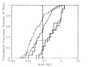
One of the main issues Matthew was investigating was whether radiative feedback had any effect on the initial mass function of the stars in his calculations. The key results are shown in the picture below (Figure 8 from the paper) in terms of cumulative distributions of the star masses in various different situations.

untitled

The question that arises from such data is whether these empirical distributions differ significantly from each other or whether they are consistent with the variations that would naturally arise in different samples drawn from the same distribution. The most interesting ones are the two distributions to the right of the plot that appear to lie almost on top of each other.

Because the samples are very small (only 13 and 15 objects respectively) one can’t reasonably test for goodness-of-fit using the standard chi-squared test because of discreteness effects and because not much is known about the error distribution. To do the statistics, therefore, Matthew uses a popular non-parametric method called the Kolmogorov-Smirnov test which uses the maximum deviation D between the two distributions as a figure of merit to decide whether they match. If D is very large then it is not probable that it can have arisen from the same distribution. If it is smaller then it might have. As for what happens if it is very small then you’ll have to wait a bit.

This is an example of a standard (frequentist) hypothesis test in which the null hypothesis is that the empirical distributions are calculated from independent samples drawn from the same underlying form. The probability of a value of D arising as large as the measured one can be calculated assuming the null is true and is then the significance level of the test. If there’s only a 1% chance of it being as large as the measured value then the significance level is 1%.

So far, so good.

But then, in describing the results of the K-S test the paper states

A Kolmogorov-Smirnov (K-S) test on the …. distributions gives a 99.97% probability that the two IMFs were drawn from the same underlying distribution (i.e. they are statistically indistinguishable).

Agh! No it doesn’t! What it gives is a probability of 99.97% that the chance deviation between the two distributions is expected to be larger than that actually measured. In other words, the two distributions are surprisingly close to each other. But the significance level merely specifies the probability that you would reject the null-hypothesis if it were correct. It says nothing at all about the probability that the null hypothesis is correct. To make that sort of statement you would need to specify an alternative distribution, calculate the distribution of D based on it, and hence determine the statistical power of the test. Without specifying an alternative hypothesis all you can say is that you have failed to reject the null hypothesis.

Or better still, if you have an alternative hypothesis you can forget about power and significance and instead work out the relative probability of the two hypotheses using a proper Bayesian approach.

You might also reasonably ask why might D be so very small? If you find an improbably low value of chi-squared then it usually means either that somebody has cheated or that the data are not independent (which is assumed for the basis of the test). Qualitatively the same thing happens with a KS test.

In fact these two distributions can’t be thought of as independent samples anyway as they are computed from the same initial conditions but with various knobs turned on or off to include different physics. They are not “samples” drawn from the same population but slightly different versions of the same sample. The probability emerging from the KS machinery is therefore meaningless anyway in this context.

So a correct statement of the result would be that the deviation between the two computed distributions is much smaller than one would expect to arise from two independent samples of the same size drawn from the same population.

That’s a much less dramatic statement than is contained in the paper, but has the advantage of not being bollocks.

Cerebral Asymmetry: is it all in the Mind?

Posted in Bad Statistics, Science Politics with tags , , on November 12, 2008 by telescoper

After blogging a few days ago about the possibility that our entire Universe might be asymmetric, I found out today that a short comment of mine about a completely different form of asymmetry has been published in the Proceedings of the National Academy of Sciences of New York.

Earlier this summer a paper by Ivanka Savic & Per Lindstrom concerning gender and sexuality differences in brain structure received widespread press coverage and the odd blog comment. They had analysed a group of 90 volunteers divided into four classes based on gender and sexual orientation: male heterosexual, male homosexual, female heterosexual and female homosexual.

They studied the brain structure of these volunteers using Magnetic Resonance Imaging and used their data to look for differences between the different classes. In particular they measured the asymmetry between left and right hemispheres for their samples. The right side of the brain for heterosexual men was found to be typically about 2% larger than the left; homosexual women also had an asymmetry, but slightly smaller than this at about 1%. Gay men and heterosexual women showed no discernible cerebral asymmetry. These claims are obviously very interesting and potentially important if they turn out to be true. It is in the nature of the scientific method that such results should be subjected to rigorous scrutiny in order to check their credibility.

As someone who knows nothing about neurobiology but one or two things about statistics, I dug out the research paper by Savic & Lindstrom and looked at the analysis it presents. I very quickly began to suspect there might be a problem. For each volunteer, the authors obtain measurements of the left and right cerebral volumes (call these L and R respectively). Each pair of measurements is then combined to form an asymmetry index (AI) as (L-R)/(L+R). There is then a set of values for AI, one for each volunteer. The claim is that these are systematically different for the different gender and orientation groups, based on a battery of tests including Analysis of Variance (ANOVA) and t-tests based on sample means.

Of course, it would be better to do this using a consistent, Bayesian, approach because this would make explicit the dependence of the results on an underlying model of the data. Sadly, the statistical methodology available off-the-shelf is of inferior frequentist type and this is what researchers tend to do when they don’t really know what they’re doing. They also don’t bother to read the health warnings that state the assumptions behind the results.

The problem in this case is that the tests done by Savic & Lindstrom all depend on the quantity being analysed (AI) having a normal (Gaussian) distribution. This is very often a reasonable hypothesis for biometric data, but unfortunately in this case the construction of the asymmetry index is such that it is expected to have a very non-Gaussian shape as is commonly the case for distributions of variables formed as ratios. In fact, the ratio of two normal variates has a peculiar distribution with very long tails. Many statistical analyses appeal to the Central Limit Theorem to justify the assumption of normality, but distributions with very long tails (such as the Cauchy distribution) violate the conditions of this Theorem, namely that the distribution must have finite variance. The asymmetry index is probably therefore an inappropriate choice of variable for the tests that Savic & Lindstrom perform. In particular the significance levels (or p-values) quoted in their paper are very low (of order 0.0008, for example, in the ANOVA test) which is surprising for such small samples. These probabilities are obtained by assuming the observations have Gaussian statistics, and they would be much lower for a distribution with longer tails.

Being a friendly chap I emailed Dr Savic drawing this problem to her attention and asking if she knew about this problem and the possible implications it might have for the analysis she had presented. If not, I offered to do an independent (private) check on the data to see how reliable the claimed statistical results actually were. I never received a reply.

Worried that the world might be jumping to all kinds of far-reaching conclusions about gay genes based on these questionable statistics, I wrote instead to the editor of the Journal Proceedings of the National Academy of Sciences of New York, Randy Schekman, who suggested I submit a written comment to the Journal. I did, it was accepted by the editorial committee, and it came out in the 11th November Issue. What I didn’t realise was that Savic & Lindstrom had actually prepared a reply and that this was published alongside my comment. I find it strange that I wasn’t told about this before publication but that aside, it is in principle quite reasonable to let the authors respond to criticisms like mine. Their response reveals that they completely missed the point of the danger of long-tailed distributions I mentioned above. They state that “when the sample size n is big the sampling distribution of the mean becomes approximately normal regardless of the distribution of the original variable“. Not if the distribution of the original variable has such a long tail it doesn’t! In fact, if the observations have a Cauchy distribution then so does the sampling distribution of the mean, whatever the size of sample. You can find this caveat spelled out in many places, including here. Savic & Lindstrom seem oblivous to this pitfall, even after I specifically pointed it out to them.

They also claim that a group size of n=30 is sufficient to be confident that the central limit theorem holds. A pity, then, that none of their groups is of that size. The overall sample is 90, but it is broken down into two groups of 20 and two of 25.

cerebral-asymmetry

(c) 2008 Academy of Sciences of New York

They also say that the measured AI distribution is actually normal anyway and give a plot (above). This shows all the AI values binned into one histogram. Since they don’t give any quantitative measures of goodness of fit, it’s hard to tell whether this has a normal distribution or not. One can, however, easily identify a group of five or six individuals that seem to form a separate group with larger AI values (the small peak to the right of the large peak). Since they don’t give histograms broken down by group it is impossible to be sure, but I would hazard a guess that these few individuals might be responsible for the entire result; remember that the entire sample has n only of 90.

More alarmingly, Savic & Lindstrom state in their reply that “one outlier” is omitted from this graph. Really? On what basis was the outlier rejected? The existence of outliers could be evidence of exactly the sort of problem I am worried about! Unless there was a known mistake in the measurement, this outlier should never have been omitted. They claim that the “recalculation of the data excluding this outlier does not change the results”. It find it difficult to believe that the removal of an outlier from such a small sample could not change the p-values!

In my note I made a few constructive suggestions as to how the difficulty might be circumvented, by Savic & Bergstrom have not followed any of them. Instead they report (without details of the p-values) having done some alternative, non-parametric, tests. These are all very well, but they don’t add very much if their p-values also assume Gaussian statistics. A better way to do this sort of thing robustly would be using Monte Carlo simulations.

The bottom line is that after this exchange of comments we haven’t really got anywhere and I still don’t know if the result is significant. I don’t really think it’s useful to go backwards and forwards through the journal, so I’ve emailed Dr Savic again asking for access to the numbers so I can check the statistics privately. In astronomy it is quite normal for people to make their data sets publically available, but that doesn’t seem to be the case in neurobiology. I’m not hopeful that they will reply, especially since they branded my comments “harsh” and “inappropriate”. Scientists should know how to take constructive criticism.

Their conclusion may eventually turn out to be right, but the analysis done so far is certainly not robust and it needs further checking. In the meantime I don’t just have doubts about the claimed significance of this specific result, which merely serves to illustrate the extremely poor level of statistical understanding displayed by large numbers of professional researchers. This was one of the things I wrote about in my book From Cosmos to Chaos. I’m very confident that a large fraction of claimed results in biosciences are based on bogus analyses.

I’ve long thought that scientific journals that deal with subjects like this should employ panels of statisticians to do the analysis independently of the authors and also that publication of the paper should require publication of the raw data. Science advances when results are subject to open criticism and independent analysis. I sincerely hope that Savic & Lindstrom will release their data in order for their conclusions to be checked in this way.

It’s no wonder that there is so much public distrust of science, when such important claims are rushed into the public domain without proper scrutiny.

A Lop-sided Universe?

Posted in Bad Statistics, Cosmic Anomalies, The Universe and Stuff with tags , on November 9, 2008 by telescoper

Over on cosmic variance, I found an old post concerning the issue of whether there might be large-scale anomalies in the cosmic microwave background sky. I blogged about this some time ago, under the title of Is there an Elephant in the Room?, so it’s interesting to see a different take on it. Interest in this issue has been highlighted by a recent paper by Groeneboom & Eriksen that claims to have detected asymmetry in the distribution of fluctuations in the data from the Wilkinson Microwave Anisotropy Probe (WMAP) inconsistent with the predictions of the standard cosmological model. If this feature is truly of primordial origin then it is an extremely important discovery as it will (probably) require the introduction of new physics into our understanding of cosmology, and that will be exciting.

It is the job of theorists to invent new theories, and it is not at all a problem that these bits of evidence have generated a number of speculative ideas. Who knows? One of them may be right. I think it is the job of theoreticians to think as radically as possible about things like this. On the other hand, it is the observational evidence that counts in the end and we should be very conservative in how we treat that. This is what bothers me about this particular issue.

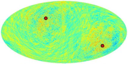
elongatedThe picture on the left shows a processed version of the WMAP fluctuation pattern designed to reveal the asymmetry, with the apparent preferred direction shown in red. This map shows the variation of the across the whole sky, and the claimed result is that the fluctuations are a bit larger around the red dots (which are 180 degrees apart) than in the regions at right angles to them.

It’s a slight effect, but everything in the picture is a slight effect as the CMB is extremely smooth to start with, the fluctuations in temperature being only about one part in a hundred thousand. The statistical analysis looks to me to be reasonably solid, so lets suppose that the claim is correct.scan

The picture on the right (courtesy of NASA/WMAP Science Team) shows the scan strategy followed by the WMAP satellite on the same projection of the sky. The experiment maps the whole sky by spinning its detectors in such a way that they point at all possible positions. The axis of this spin is chosen in a particular way so that it is aligned with the ecliptic poles (out of the plane of the solar system). It is in the nature of this procedure that it visits some places more than others (those at the ecliptic poles are scanned more often than those at the equator), hence the variation in signal-to-noise shown in the map. You can see that effect graphically in the picture: the regions near the North and South ecliptic poles have better signal to noise than the others.

The axis found by Groeneboom & Eriksen is not perfectly aligned with the ecliptic plane but it is pretty close. It seems a reasonable (if conservative) interpretation of this that the detected CMB anomaly could be due to an unknown systematic that has something to do either with the solar system (such as an unknown source of radiation, like cold dust) or the way the satellite scans. The WMAP team have worked immensely hard to isolate any such systematics so if this is such an effect then it must be very subtle to have escaped their powerful scrutiny. They’re all clever people and it’s a fabulous experiment, but that doesn’t mean that it is impossible that they have missed something.

Many of the comments that have been posted on cosmic variance relating to this question the statistical nature of the result. Of course we have only one sky available, so given the “randomness” of the fluctuations it is possible that freakish configurations occur by chance. This misses the essentially probabilistic nature of all science which I tried to describe in my book on probability From Cosmos to Chaos. We are always limited by noise and incompleteness but that doesn’t invalidate the scientific method. In cosmology these problems are writ large because of the nature of the subject, but there is no qualitative difference in the interplay between science and theory in cosmology compared with other sciences. It’s just less easy to get the evidence.

So the issue here, which is addressed only partially by Groeneboom % Eriksen, is whether a lop-sided universe is more probable than an isotropic one given the WMAP measurements. They use a properly consistent Bayesian argument to tackle this issue and form a reasonably strong conclusion that the answer is yes. As far as it goes, I think this is (probably) reasonable.

However, now imagine I don’t believe in anistropic cosmologies but instead have an idea that this is caused by an unknown systematic relating in some way to the ecliptic plane. Following the usual Bayesian logic I think it is clear that, although both can account for the data, my hypothesis must be even more probable than a lop-sided universe. There is no reason why a primordial effect should align so closely with the ecliptic plane, so there is one unexplained coincidence in the lop-sided-universe model, whereas my model neatly accounts for that fact without any freedom to adjust free parameters. Ockham’s razor is on my side.

So what can we do about this? The answer might be not very much. It is true that, soon, the Planck Surveyor will be launched and it will map the CMB sky againat higher resolution and sensitivity. On the other hand, it will not solve the problem that we only have one sky. The fact that it is a different experiment may yield clues to any residual systematics in the WMAP results, but if it has a similar scan strategy to WMAP, even Planck might not provide definitive answers.

I think this one may run and run!

The Curious Case of the Inexpert Witness

Posted in Bad Statistics with tags , , , on September 17, 2008 by telescoper

Although I am a cosmologist by trade, I am also interested in the fields of statistics and probability theory. I guess this derives from the fact that a lot of research in cosmology depends on inferences drawn from large data sets. By its very nature this process is limited by the fact that the information obtained in such studies is never complete. The analysis of systems based on noisy or incomplete data is exactly what probability is about.

Of course, statistics has much wider applications than in pure science and there are times when it is at the heart of controversies that explode into the public domain, particularly when involved in medicine or jurisprudence. One of the reasons why I wrote my book From Cosmos to Chaos was a sense of exasperation at how poorly probability theory is understood even by people who really should know better. Although statistical reasoning is at the heart of a great deal of research in physics and astronomy, there are many prominent practioners who don’t really know what they are talking about when they discuss probability. As I soon discovered when I started thinking about writing the book, the situation is even worse in other fields. I thought it might be fun to post a few examples of bad statistics from time to time, so I’ll start with this, which is accompanied by a powerpoint file of a lunchtime talk I gave at Cardiff.

I don’t have time to relate the entire story of Sally Clark and the monstrous miscarriage of justice she endured after the deaths of her two children. The wikipedia article I have linked to is pretty accurate, so I’ll refer you there for the details. In a nutshell, in 1999 she was convicted of the murder of her two children on the basis of some dubious forensic evidence and the expert testimony of a prominent paediatrician, Sir Roy Meadow. After appeal her convinction was quashed in 2003, but she died in 2007 from alcohol poisoning having apparently taken to the bottle after three years of wrongful imprisonment.

Professor Meadow had a distinguished (if somewhat controversial) career, becoming famous for a paper on Munchausen’s Syndrome by Proxy which appeared in the Lancet in 1977. He subsequently appeared as an expert witness in many trials of parents accused of murdering their children. In the Sally Clark case he was called as a witness for the prosecution, where his testimony included an entirely bogus and now infamous argument about the probability of two sudden infant deaths happening accidentally in the same family.

The argument is basically the following. The observed ratio of live births to cot deaths in affluent non-smoking families (like Sally Clark’s) is about 8,500:1. This means that about 1 in 8,500 children born to such families die in such a way. He then argued that the probability that two such tragedies happen in the same family is this number squared, i.e. about 73,000,000:1. In the mind of the jury this became the odds against the death of Mrs Clark’s children being accidental and therefore presumably the odds against her being innocent. The jury found her guilty.

For reasons why this argument is completely bogus, and more technical details, look in the following powerpoint file (which involves a bit of maths):

the-inexpert-witness

It is difficult to assess how important Roy Meadow’s testimony was in the collective mind of the Jury, but it was certainly erroneous and misleading. The General Medical Council decided that he should be struck off the medical register in July 2005 on the grounds of “serious professional misconduct”. He appealed, and the decision was partly overturned in 2006, the latest judgement basically being about what level of professional misconduct should be termed “serious”.

My reaction to all this is a mixture of anger and frustration. First of all, the argument presented by Meadow is so clearly wrong that any competent statistician could have been called as a witness to rebut it. The defence were remiss in not doing so. Second, the disciplinary action taken by the GMC seemed to take no account of the consequences his testimony had for Sally Clark. He was never even at risk of prosecution or financial penalty. Sally Clark spent three years of her life in prison, on top of having lost her children, and now is herself dead. Finally, expert testimony is clearly important in many trials, but experts should testify only on those matters that they are experts about! Meadow even admitted later that he didn’t really understand statistics. So why did he include this argument in his testimony? I quote from a press release produced by the Royal Statistical Society in the aftermath of this case:

Although many scientists have some familiarity with statistical methods, statistics remains a specialised area. The Society urges the Courts to ensure that statistical evidence is presented only by appropriately qualified statistical experts, as would be the case for any other form of expert evidence.

As far as I know, the criminal justice system has yet to implement such safeguards.

How many more cases like this need to happen before the Courts recognise the dangers of bad statistics?