Archive for Cosmic Microwave Background

The Cold Spot

Posted in Cosmic Anomalies, The Universe and Stuff with tags , , , , on August 16, 2009 by telescoper

Musing yesterday about the rapidly approaching restart of the academic year reminded me that I really ought to get on and finish the bunch of papers sitting on my desk and on various computers. I’ve also got a book to finish before October so I’d better get cracking with that too.

More importantly, however, it reminded me to congratulate my PhD student Rockhee Sung who has just had her first paper published (in the journal Classical and Quantum Gravity). The paper is available online here and it’s free to download for a month even if you don’t have a personal or institutional subscription to the journal.

The idea of this paper came a while ago but it has taken us a long time to get everything in place to start writing it up. In the meantime other papers have been written on the subject, but Rockhee and I have done this our own way – or rather she has, as she put most of the hard work into actually doing the calculations.

About four years ago, during the course of careful statistical analysis of data from the Wilkinson Microwave Anisotropy Probe (WMAP), a group based in Santander (Spain) published a paper drawing attention to the existence of an anomalous “Cold Spot” in the data. This phenomenon has now acquired its own Wikipedia entry (here), so I won’t repeat all the details except to say that it is about 5° across and that it is colder than one would expect if the temperature fluctuations are Gaussian, as is predicted in the simplest models of the early Universe involving cosmological inflation. The spot is to the bottom right, and is marked with an arrow on the picture below.

It’s worth digressing a little here to explain that a fluctuating field of course contains both hot spots and cold spots. Because there CMB temperature fluctuations comprise a wide range of wavelengths there are also spots on different scales. Assessing the statistical significance of a single isolated feature like the cold spot is not particularly easy. Based on the brute force method of simulating skies according to the Gaussian hypothesis and then repeating the approach that led to the original discovery, the result is that around 1% of Gaussian CMB skies have a cold spot as cold as that observed in the real data. Before the non-Bayesians among you get too excited, I’ll remind you that this means that the probability of a Cold spot given the standard model is about 1%, i.e. P(Cold Spot | Standard Model)=0.01. This is NOT the same as saying that the probability of the standard model being correct is 0.01…

A probability of 1% is an in-between kind of level: not too small to be decisive, and not too large to be instantly dismissed as just being a chance fluctuation. My personal opinion is that the Cold Spot is an interesting feature that deserves to be investigated further, but is not something that in itself should cause anyone to doubt the standard model. I include it among the list of cosmological anomalies that I’ve blogged about before (for example, here, here and here). I find them interesting but don’t lose sleep worrying that the standard model is about to fall to pieces. Not yet, anyway.

Not all theorists are as level-headed as me, however, and within weeks of the discovery of the cold spot suggestions were already being put forward as to how it could be “explained” theoretically. Some of these are described in the Wikipedia entry, so I won’t rehash the list. However, one suggestion not included there was the idea that the anomalous cold spot might be there because the Universe were not isotropic, i.e. if the Cosmological Principle were violated.

Way back when I was a lad doing my own PhD, my supervisor John Barrow had been interested in globally anisotropic (but nevertheless homogeneous) cosmologies. These are models in which any observer sees different things in different directions, but the pattern seen by observers in different places is always the same. I never worked on these at the time – they seemed a bit too esoteric even for me – but I remembered bits and pieces about them from conversations.

A complete classification of all the space-times  possessing this property was completed over a hundred years ago (before General Relativity was invented) by the Italian mathematician Luigi Bianchi, and cosmological models based on them are called the Bianchi models.

This isn’t the place to go into detail about the Bianchi models: the classification is based on the mathematical properties of Lie groups, which would take me ages to explain. However, it is worth pointing out that only five Bianchi types actually contain the cosmologically principled Friedmann-Lemaître-Robertson-Walker universe as a special case: I, V, VII0 ,VIIh and IX. If you really want to know what the classes are you’ll have to look them up! Since we know our Universe is very close to being homogeneous and isotropic, it seems reasonable to look at those models capable of describing small departures from that case so the above list provides a useful subset of the models to explore.

Rockhee’s PhD project was to explore  the patterns of cosmic microwave background  fluctuations that can arise in that set of Bianchi cosmologies, not just in the temperature (which had been done before) but also in polarization (which hadn’t). I’ve already posted some of the temperature patterns Rockhee computed here.

The reason for extending wanting to extend this work to include polarization was the following. The microwave background radiation is partly linearly polarized because of the way radiation is scattered by electrons. If an electron is immersed in a radiation bath which is isotropic there is no net polarization, but if the radiation field is anisotrpic – in particular if it varies on an angular scale of 90º (i.e. a quadrupole) – then the scattered radiation will be partly polarized. In the standard cosmology the variations in the radiation field are random fluctuations so each electron “sees” a different quadupole. The net polarization field is therefore produced incoherently, by adding stochastic contributions. In  a  Bianchi model the situation is different. Each electron in this case sees the same quadupole. The polarization pattern produced is therefore coherent. Not only do anisotropic universes produce characteristic radiation patterns, they also produce a corresponding pattern in polarization.

So what does this all have to do with the Cold Spot? Well, in anisotropic spaces that are also curved, it is possible for light rays to get focussed in such a way that the entire pattern of flucuations present at least-scattering winds up concentrated in a small patch of the sky as seen by a late-time observer. for this to happen the space has to be negatively curved. Only two of the Bianchi types can do this, as there are only two that are both near-FLRW and negatively curved: V and VIIh. Both of these models could, in principle, therefore produce a cold spot by geometrical, rather than stochastic means. In the little figure below, taken from our paper, you can see examples of Bianchi VIIh (top) and Bianchi V (bottom) showing the temperature (left) and polarization (right) in each case. We’ve oriented the model to put the cold spot in approximately the right location as the observed one.


cold


The point is that there is a pretty heavy price to be paid for producing the cold spot in this way: an enormous, coherent signal in the polarized radiation field.

As often happens in such situations, somebody else had the idea to investigate these models and we were scooped to a large extent by Andrew Pontzen and Anthony Challinor from Cambridge, who recently published a paper showing that the polarization produced in these models is already excluded by experimental upper limits. They concentrated on the Bianchi VIIh case, as this appears to have a more general structure than V and it was the model first advocated as an explanation of the cold spot. In this model the combined effect of vorticity and shear introduces a swirly pattern into the radiation field that you can see clearly in the top two panels of the figure as well as focussing it into a small patch. Bianchi V doesn’t produce the same kind of pattern either in temperature or polarization: it looks more like a simple quadrupole squeezed into a small part of the sky. A particularly interesting aspect of this is that the Bianchi VIIh case clearly has a definite “handedness” while the Bianchi V one doesn’t.

The moral of all this is that the polarization of the cosmic microwave background provides key additional information that could prove decisive in eliminating (or perhaps even confirming) models of the Universe more exotic than the standard one. That’s one of the areas in which  we expect Planck to produce the goods!

In the meantime Rockhee and I will be submitting a couple of much larger papers in due course, one containing a wider discussion of the possible pattern morphologies that can be produced in these models, and another about their detailed statistical properties.

The Axle of Elvis

Posted in Cosmic Anomalies, The Universe and Stuff with tags , , , , , , on August 6, 2009 by telescoper

An interesting paper on the arXiv yesterday gave me a prod to expand a little on one of the cosmic anomalies I’ve blogged about before.

Before explaining what this is all about, let me just briefly introduce a bit of lingo. The pattern of variations fluctuations in the temperature of the cosmic microwave background (CMB) across the sky, such as is revealed by the Wilkinson Microwave Anisotropy Probe (WMAP), is usually presented in terms of the behaviour of its spherical harmonic components. The temperature as a function of position is represented as a superposition of spherical harmonic modes labelled by two numbers, the degree l and the order m. The degree basically sets the characteristic angular scale of the mode (large  scales have low l, and small scales have high l). For example the dipole mode has l=1 and it corresponds to variation across the sky on a scale of 180 degrees; the quadrupole (l=2) has a scale of 90 degrees, and so on. For a fixed l the order m runs from -l to +l and each order represents a particular pattern with that given scale.

The spherical harmonic coefficients that tell you how much of each mode is present in the signal are generally  complex numbers having real and imaginary parts or, equivalently, an amplitude and a phase.  The exception to this are the modes with m=0, the zonal modes, which have no azimuthal variation: they vary only with latitude, not longitude. These have no imaginary part so don’t really have a phase. For the other modes, the phase controls the variation with azimuthal angle around the axis of the chosen coordinate system, which in the case of the CMB is usually taken to be the Galactic one.

In the simplest versions of cosmic inflation, each of the spherical harmonic modes should be statistically independent and randomly distributed in both amplitude and phase. What this really means is that the harmonic modes are in a state of maximum statistical disorder or entropy. This property also guarantees that the temperature fluctuations over the sky should be described by  a Gaussian distribution.

That was perhaps a bit technical but the key idea is that if you decompose the overall pattern of fluctuations into its spherical harmonic components the individual mode patterns should look completely different. The quadrupole and octopole, for example, shouldn’t line up in any particular way.

Evidence that this wasn’t the case started to emerge when WMAP released its first set of data in 2003 with indications of an alignment between the modes of low degree. In their  analysis, Kate Land and Joao Magueijo dubbed this feature The Axis of Evil; the name has stuck.They concluded that there was a statistically significant alignment (at 99.9% confidence) between the multipoles of low degree (l=2 and 3), meaning that the measured alignment is only expected to arise by chance in one in a thousand simulated skies. More recently, further investigation of this effect using subsequent releases of data from the WMAP experiment and a more detailed treatment of the analysis (including its stability with respect to Galactic cuts) suggested that the result is not quite as robust as had originally been claimed. .

Here are the low-l modes of the WMAP data so you see what we’re talking about. The top row of the picture contains the modes for l=2 (quadrupole) and l=3 (octopole) and the bottom shows l=4 and l=5.


The two small red blobs mark the two ends of the preferred axis of each mode. The orientation of this axis is consistent across all the modes shown but the statistical significance is much stronger for the ones with lower l.

It’s probably worth mentioning a couple of neglected aspects of this phenomenon. One is that the observed quadrupole and octopole appear not only to be aligned with each other but also appear to be dominated by sectoral orders, i.e those with m=l. These are the modes which are, in a sense, opposite to the zonal modes in that they vary only with longitude and not with latitude. Here’s what the sectoral mode of the quadrupole looks like:

map22

Changing the phase of this mode would result in the pattern moving to the left or right, i.e. changing its origin, but wouldn’t change the orientation. Which brings me to the other remarkable thing, namely that the two lowest modes also have  correlated phases. The blue patch to the right of Galactic centre is in the same place for both these modes. You can see the same feature in the full-resolution map (which involves modes up to l~700 or so):

I don’t know whether there is really anything anomalous about the low degree multipoles, but I hope this is a question that Planck (with its extra sensitivity, better frequency coverage and different experimental strategy) will hopefully shed some light on. It could be some sort of artifact of the measurement process or it could be an indication of something beyond the standard cosmology. It could also just be a fluke. Or even the result of an over-active imagination, like seeing Elvis in your local Tesco.

On its own I don’t think this is going to overthrow the standard model of cosmology. Introducing extra parameters to a model in order to explain a result with a likelihood that is only marginally low in a simpler model does not make sense, at least not to a proper Bayesian who knows about model selection…

However, it is worth mentioning that the Axis of Evil isn’t the only cosmic anomaly to have been reported. If an explanation is found with relatively few parameters that can account for all of these curiosities in one fell swoop then it would stand a good chance of convincing us all that there is more to the Universe than we thought. And that would be fun.

How Loud was the Big Bang?

Posted in The Universe and Stuff with tags , , , , , , on April 26, 2009 by telescoper

The other day I was giving a talk about cosmology at Cardiff University’s Open Day for prospective students. I was talking, as I usually do on such occasions, about the cosmic microwave background, what we have learnt from it so far and what we hope to find out from it from future experiments, assuming they’re not all cancelled.

Quite a few members of staff listened to the talk too and, afterwards, some of them expressed surprise at what I’d been saying, so I thought it would be fun to try to explain it on here in case anyone else finds it interesting.

As you probably know the Big Bang theory involves the assumption that the entire Universe – not only the matter and energy but also space-time itself – had its origins in a single event a finite time in the past and it has been expanding ever since. The earliest mathematical models of what we now call the  Big Bang were derived independently by Alexander Friedman and George Lemaître in the 1920s. The term “Big Bang” was later coined by Fred Hoyle as a derogatory description of an idea he couldn’t stomach, but the phrase caught on. Strictly speaking, though, the Big Bang was a misnomer.

Friedman and Lemaître had made mathematical models of universes that obeyed the Cosmological Principle, i.e. in which the matter was distributed in a completely uniform manner throughout space. Sound consists of oscillating fluctuations in the pressure and density of the medium through which it travels. These are longitudinal “acoustic” waves that involve successive compressions and rarefactions of matter, in other words departures from the purely homogeneous state required by the Cosmological Principle. The Friedman-Lemaitre models contained no sound waves so they did not really describe a Big Bang at all, let alone how loud it was.

However, as I have blogged about before, newer versions of the Big Bang theory do contain a mechanism for generating sound waves in the early Universe and, even more importantly, these waves have now been detected and their properties measured.

The above image shows the variations in temperature of the cosmic microwave background as charted by the Wilkinson Microwave Anisotropy Probe about five years ago. The average temperature of the sky is about 2.73 K but there are variations across the sky that have an rms value of about 0.08 milliKelvin. This corresponds to a fractional variation of a few parts in a hundred thousand relative to the mean temperature. It doesn’t sound like much, but this is evidence for the existence of primordial acoustic waves and therefore of a Big Bang with a genuine “Bang” to it.

A full description of what causes these temperature fluctuations would be very complicated but, roughly speaking, the variation in temperature you corresponds directly to variations in density and pressure arising from sound waves.

So how loud was it?

The waves we are dealing with have wavelengths up to about 200,000 light years and the human ear can only actually hear sound waves with wavelengths up to about 17 metres. In any case the Universe was far too hot and dense for there to have been anyone around listening to the cacophony at the time. In some sense, therefore, it wouldn’t have been loud at all because our ears can’t have heard anything.

Setting aside these rather pedantic objections – I’m never one to allow dull realism to get in the way of a good story- we can get a reasonable value for the loudness in terms of the familiar language of decibels. This defines the level of sound (L) logarithmically in terms of the rms pressure level of the sound wave Prms relative to some reference pressure level Pref

L=20 log10[Prms/Pref]

(the 20 appears because of the fact that the energy carried goes as the square of the amplitude of the wave; in terms of energy there would be a factor 10).

There is no absolute scale for loudness because this expression involves the specification of the reference pressure. We have to set this level by analogy with everyday experience. For sound waves in air this is taken to be about 20 microPascals, or about 2×10⁻¹⁰ times the ambient atmospheric air pressure which is about 100,000 Pa.  This reference is chosen because the limit of audibility for most people corresponds to pressure variations of this order and these consequently have L=0 dB. It seems reasonable to set the reference pressure of the early Universe to be about the same fraction of the ambient pressure then, i.e.

Pref~2×10⁻¹⁰ Pamb

The physics of how primordial variations in pressure translate into observed fluctuations in the CMB temperature is quite complicated, and the actual sound of the Big Bang contains a mixture of wavelengths with slightly different amplitudes so it all gets a bit messy if you want to do it exactly, but it’s quite easy to get a rough estimate. We simply take the rms pressure variation to be the same fraction of ambient pressure as the averaged temperature variation are compared to the average CMB temperature,  i.e.

Prms~ a few ×10-5Pamb

If we do this, scaling both pressures in logarithm in the equation in proportion to the ambient pressure, the ambient pressure cancels out in the ratio, which turns out to be a few times 10-5.

AudiogramsSpeechBanana

With our definition of the decibel level we find that waves corresponding to variations of one part in a hundred thousand of the reference level  give roughly L=100dB while part in ten thousand gives about L=120dB. The sound of the Big Bang therefore peaks at levels just over  110 dB. As you can see in the Figure above, this is close to the threshold of pain,  but it’s perhaps not as loud as you might have guessed in response to the initial question. Many rock concerts are actually louder than the Big Bang, at least near the speakers!

A useful yardstick is the amplitude  at which the fluctuations in pressure are comparable to the mean pressure. This would give a factor of about 1010 in the logarithm and is pretty much the limit that sound waves can propagate without distortion. These would have L≈190 dB. It is estimated that the 1883 Krakatoa eruption produced a sound level of about 180 dB at a range of 100 miles. By comparison the Big Bang was little more than a whimper.

PS. If you would like to read more about the actual sound of the Big Bang, have a look at John Cramer’s webpages. You can also download simulations of the actual sound. If you listen to them you will hear that it’s more of  a “Roar” than a “Bang” because the sound waves don’t actually originate at a single well-defined event but are excited incoherently all over the Universe.

Ecliptic Anomalies

Posted in Cosmic Anomalies, The Universe and Stuff with tags , , , , on February 12, 2009 by telescoper

Once a week the small band of cosmologists at Cardiff University have a little discussion group during which we look at an interesting and topical subject. Today my PhD student Rockhee chose an interesting paper by Diego et al entitled “WMAP anomalous signal in the ecliptic plane”. I thought I’d mention it here because it relates to an ongoing theme of mine, and I’ll refrain from commenting on the poor grammatical construction of the title.

The WMAP referred to is of course the Wilkinson Microwave Anisotropy Probe and I’ve blogged before about the tantalising evidence it suggests of some departures from the standard cosmological theory. These authors do something very simple and the result is extremely interesting.

In order to isolate the cosmic microwave background from foreground radiation produced in our own Galaxy, the WMAP satellite is equipped with receivers working at different frequencies. Galactic dust and free-free emission dominate the microwave sky temperature at high frequencies and Galactic synchotron takes over at low frequencies. The cosmic microwave background has the same temperature at all frequencies (i.e. it has a thermal spectrum) so it should be what’s left when the frequency-dependent bits are cleaned out.

What Diego et al. did was to make a map by combining the cleaned sky maps obtained at different frequencies obtained by WMAP in such a way as to try to eliminate the thermal (CMB) component. What is left when this is done should be just residual noise, as it should contain neither known foreground or CMB. The map they get is shown here.ecliptic

What is interesting is that the residual map doesn’t look like noise that is uniformly distributed over the sky: there are two distinct peaks close to the Ecliptic plane delineated by the black tramlines. Why the residuals look like this is a mystery. The peaks are both very far from the Galactic plane so it doesn’t look like they are produced by Galactic foregrounds.

One suggestion is that the anomalous signal is like an infra-red extension of the Zodiacal light (which is produced inside the Solar System and therefore is too local to be confined to the Galactic plane). The authors show, however, that a straightforward extrapolation of the known Zodiacal emission (primarily measured by the IRAS satellite) does not account for the signal seen in WMAP. If this is the explanation, then, there has to be a new source of Zodiacal emission that is not seen by IRAS but kicks in at WMAP frequencies.

Another possibility is that it is extragalactic. This is difficult to exclude, but is disfavoured in my mind because there is no a priori reason why it should be concentrated in the Ecliptic plane. Coincidences like this make me a bit uncomfortable. Some turn out to be real coincidences, but more often than not they are clues to something important. Agatha Christie would have agreed:

“Any coincidence,” said Miss Marple to herself, “is always worth noting. You can throw it away later if it is only a coincidence.”

On the other hand, the dipole asymmetry of the CMB (thought to be caused by our motion through a frame in which it is isotropic) is also lined up in roughly the same direction:

The dipole has a hot region and a cold region in places where the residual map has two hot regions and anyway it’s also a very large scale feature so the chances of it lining up by accident with the ecliptic plane to the accuracy seen is actually not small. Coincidences definitely do happen, and the rougher they are the more commonly they occur.

Obviously, I don’t know what’s going on, but  I will mention another explanation that might fit. As I have already blogged, the WMAP satellite scans the sky in a way that is oriented exactly at right angles to the Ecliptic plane. If there is an as yet unknown systematic error in the WMAP measurements, which is related in some way to the motion of the satellite, it could at least in principle produce an effect with a definite orientation with respect to the Ecliptic.

The only way we can rule out this (admittedly rather dull) explanation is by making a map using a different experiment. It’s good, then, that the Planck satellite is going to be launched in only a few weeks’ time (April 16th 2009). Fingers crossed that we can solve this riddle soon.

Power isn’t Everything

Posted in The Universe and Stuff with tags , , , , , , , on January 6, 2009 by telescoper

WMapThe picture above shows the latest available all-sky map of fluctuations in the temperature of the cosmic microwave background across the sky as revealed by the Wilkinson Microwave Anisotropy Probe, known to its friends as WMAP.

I’ve spent many long hours fiddling with the data coming from the WMAP experiment, partly because I’ve never quite got over the fact that such wonderful data actually exists. When I started my doctorate in 1985 the whole field of CMB analysis was so much pie in the sky, as no experiments had yet been performed with the sensitivity to reveal the structures we now see. This is because they are very faint and easily buried in noise. The fluctuations in temperature from pixel to pixel across the sky are of order one part in a hundred thousand of the mean temperature (i.e. about 30 microKelvin on a background temperature of about 3 Kelvin). That’s smoother than the surface of a billiard ball. That’s why it took such a long time to make the map shown above, and why it is such a triumphant piece of science.

I blogged a few days ago about the idea that the structure we see in this map was produced by sound waves reverberating around the early Universe. The techniques cosmologists use to analyse this sound are similar to those used in branches of acoustics except that we only see things in projection on the celestial sphere which requires a bit of special consideration.

One of the things that sticks in my brain from my undergraduate years is being told that if a physicist doesn’t know what they are doing they should start by making a Fourier transform. This breaks down the phenomenon being studied into a set of independent plane waves with different wavelengths corresponding to the different tones present in a complicated sound.

It’s often very good advice to do such a decomposition for one-dimensional time series or fluctuation fields in three-dimensional Cartesian space, even you do know what you’re doing, but it doesn’t work with a sphere because plane waves don’t fit properly on a curved surface. Fortunately, however, there is a tried-and-tested alternative involving spherical harmonics rather than plane waves.

Spherical harmonics are quite complicated beasts mathematically but they have pretty similar properties to Fourier harmonics in many respects. In particular they are represented as complex numbers having real and imaginary parts or, equivalently, an amplitude and a phase (usually called an argument by mathematicians). The latter representation is the most useful one for CMB fluctuations because the simplest versions of inflation predict that the phases of each of the spherical harmonic modes should be randomly distributed. What this really means is that there is no information content in their distribution so that the harmonic modes are in a state of maximum statistical disorder or entropy. This property also guarantees that the distribution of fluctuations over the sky should have a Gaussian distribution.

If you accept that the fluctuations are Gaussian then only the amplitudes of the spherical harmonic coefficients are useful. Indeed, their statistical properties can be specified entirely by the variance of these amplitudes as a function of mode frequency. This pre-eminently important function is called the power-spectrum of the fluctuations, and it is shown here for the WMAP data:

080999_powerspectrumm

Although the units on the axes are a bit strange it doesn”t require too much imagination to interpret this in terms of a sound spectrum. There is a characteristic tone (at the position of the peak) plus a couple of overtones. However these features are not sharp so the overall sound is not at all musical.

If the Gaussian assumption is correct then the power-spectrum contains all the useful statistical information to be gleaned from the CMB sky, which is why so much emphasis has been placed on extracting it accurately from the data.

Conversely, though, the power spectrum is completely insenstive to any information in the distribution of spherical harmonic phases. If something beyond the standard model made the Universe non-Gaussian it would affect the phases of the harmonic modes in a way that would make them non-random.

So far, so good. It sounds like it should be a straightforward job to work out whether the WMAP phases are random or not. Unfortunately, though, this task is heavily complicated by the presence of noise and systematics which can be quite easily cleaned from the spectrum but not from more sophisticated descriptors. All we can say so far is that the data seem to be consistent with a Gaussian distribution.

However, I thought I’d end with a bit of fun and show you how important phase information could actually be, if only we could find a good way of exploiting it. Let’s start with a map of the Earth, with the colour representing height of the surface above mean sea level:

sw_world

You can see the major mountain ranges (Andes, Himalayas) quite clearly as red in this picture and note how high Antarctica is…that’s one of the reasons so much astronomy is done there.

Now, using the same colour scale we have the WMAP data again (in Galactic coordinates).

sw_ilc

The virture of this map is that it shows how smooth the microwave sky is compared to the surface of the Earth. Note also that you can see a bit of crud in the plane of the Milky Way that serves as a reminder of the difficulty of cleaning the foregrounds out.

Clearly these two maps have completely different power spectra. The Earth is dominated by large features made from long-wavelength modes whereas the CMB sky has relatively more small-scale fuzz.

Now I’m going to play with these maps in the following rather peculiar way. First, I make a spherical harmonic transform of each of them. This gives me two sets of complex numbers, one for the Earth and one for WMAP. Following the usual fashion, I think of these as two sets of amplitudes and two sets of phases. Note that the spherical harmonic transformation preserves all the information in the sky maps, it’s just a different representation.

Now what I do is swap the amplitudes and phases for the two maps. First, I take the amplitudes of WMAP and put them with the phases for the Earth. That gives me the spherical harmonic representation of a new data set which I can reveal by doing an inverse spherical transform:

sw_worldphases

This map has exactly the same amplitudes for each mode as the WMAP data and therefore possesses an identical power spectrum to that shown above. Clearly, though, this particular CMB sky is not compatible with the standard cosmological model! Notice that all the strongly localised features such as coastlines appear by virtue of information contained in the phases but absent from the power-spectrum.

To understand this think how sharp features appear in a Fourier transform. A sharp spike at a specific location actually produces a broad spectrum of Fourier modes with different frequencies. These modes have to add in coherently at the location of the spike and cancel out everywhere else, so their phases are strongly correlated. A sea of white noise also has a flat power spectrum but has random phases. The key difference between these two configurations is not revealed by their spectra but by their phases.

Fortunately there is nothing quite as wacky as a picture of the Earth in the real data, but it makes the point that there are more things in Heaven and Earth than can be described in terms of the power spectrum!

Finally, perhaps in your mind’s eye you might consider what it might look lie to do the reverse experiment: recombine the phases of WMAP with the amplitudes of the Earth.

sw_ilcphases

If the WMAP data are actually Gaussian, then this map is a sort of random-phase realisation of the Earth’s power spectrum. Alternatively you can see that it is the result of running a kind of weird low-pass filter over the WMAP fluctuations. The only striking things it reveals are (i) a big blue hole associated with foreground contamination, (ii) a suspicious excess of red in the galactic plane owing to the same problem, and (iiI) a strong North-South asymmetry arising from the presence of Antarctica.

There’s no great scientific result here, just a proof that spherical harmonics can be fun.

PS. These pictures were made by a former PhD student of mine, Patrick Dineen, who has since quit astronomy to work in high finance. I hope he is weathering the global financial storm!

Who put the Bang in Big Bang?

Posted in The Universe and Stuff with tags , , , , , on December 29, 2008 by telescoper

Back from the frozen North, having had a very nice time over Christmas, I thought it was time to reactivate my blog and to redress the rather shameful lack of science on what is supposed to be a science blog. Rather than writing a brand new post, though, I’m going to cheat like a TV Chef by sticking up something that I did earlier. I’ve  had the following piece floating around on my laptop for a while so I thought I’d rehash it and post it on here. It is based on an article that was published in a heavily revised and shortened form in New Scientist in 2007, where it attracted some splenetic responses despite there not being anything particular controversial in it! It’s not particularly topical, but there you go. The television is full of repeats these days too.

Around twenty-five years ago a young physicist came up with what seemed at first to be an absurd idea: that, for a brief moment in the very distant past, just after the Big Bang, something weird happened to gravity that made it push rather than pull.  During this time the Universe went through an ultra-short episode of ultra-fast expansion. The physicist in question, Alan Guth, couldn’t prove that this “inflation” had happened nor could he suggest a compelling physical reason why it should, but the idea seemed nevertheless to solve several major problems in cosmology.

Twenty five years later on, Guth is a professor at MIT and inflation is now well established as an essential component of the standard model of cosmology. But should it be? After all, we still don’t know what caused it and there is little direct evidence that it actually took place. Data from probes of the cosmic microwave background seem to be consistent with the idea that inflation happened, but how confident can we be that it is really a part of the Universe’s history?

According to the Big Bang theory, the Universe was born in a dense fireball which has been expanding and cooling for about 14 billion years. The basic elements of this theory have been in place for over eighty years, but it is only in the last decade or so that a detailed model has been constructed which fits most of the available observations with reasonable precision. The problem is that the Big Bang model is seriously incomplete. The fact that we do not understand the nature of the dark matter and dark energy that appears to fill the Universe is a serious shortcoming. Even worse, we have no way at all of describing the very beginning of the Universe, which appears in the equations used by cosmologists as a “singularity”- a point of infinite density that defies any sensible theoretical calculation. We have no way to define a priori the initial conditions that determine the subsequent evolution of the Big Bang, so we have to try to infer from observations, rather than deduce by theory, the parameters that govern it.

The establishment of the new standard model (known in the trade as the “concordance” cosmology) is now allowing astrophysicists to turn back the clock in order to understand the very early stages of the Universe’s history and hopefully to understand the answer to the ultimate question of what happened at the Big Bang itself and thus answer the question “How did the Universe Begin?”

Paradoxically, it is observations on the largest scales accessible to technology that provide the best clues about the earliest stages of cosmic evolution. In effect, the Universe acts like a microscope: primordial structures smaller than atoms are blown up to astronomical scales by the expansion of the Universe. This also allows particle physicists to use cosmological observations to probe structures too small to be resolved in laboratory experiments.

Our ability to reconstruct the history of our Universe, or at least to attempt this feat, depends on the fact that light travels with a finite speed. The further away we see a light source, the further back in time its light was emitted. We can now observe light from stars in distant galaxies emitted when the Universe was less than one-sixth of its current size. In fact we can see even further back than this using microwave radiation rather than optical light. Our Universe is bathed in a faint glow of microwaves produced when it was about one-thousandth of its current size and had a temperature of thousands of degrees, rather than the chilly three degrees above absolute zero that characterizes the present-day Universe. The existence of this cosmic background radiation is one of the key pieces of evidence in favour of the Big Bang model; it was first detected in 1964 by Arno Penzias and Robert Wilson who subsequently won the Nobel Prize for their discovery.

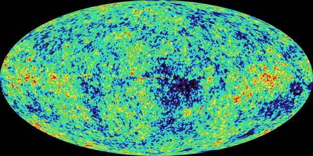
The process by which the standard cosmological model was assembled has been a gradual one, but it culminated with recent results from the Wilkinson Microwave Anisotropy Probe (WMAP). For several years this satellite has been mapping the properties of the cosmic microwave background and how it varies across the sky. Small variations in the temperature of the sky result from sound waves excited in the hot plasma of the primordial fireball. These have characteristic properties that allow us to probe the early Universe in much the same way that solar astronomers use observations of the surface of the Sun to understand its inner structure,  a technique known as helioseismology. The detection of the primaeval sound waves is one of the triumphs of modern cosmology, not least because their amplitude tells us precisely how loud the Big Bang really was.

The pattern of fluctuations in the cosmic radiation also allows us to probe one of the exciting predictions of Einstein’s general theory of relativity: that space should be curved by the presence of matter or energy. Measurements from WMAP reveal that our Universe is very special: it has very little curvature, and so has a very finely balanced energy budget: the positive energy of the expansion almost exactly cancels the negative energy relating of gravitational attraction. The Universe is (very nearly) flat.

The observed geometry of the Universe provides a strong piece of evidence that there is an mysterious and overwhelming preponderance of dark stuff in our Universe. We can’t see this dark matter and dark energy directly, but we know it must be there because we know the overall budget is balanced. If only economics were as simple as physics.

Computer Simulation of the Cosmic Web

The concordance cosmology has been constructed not only from observations of the cosmic microwave background, but also using hints supplied by observations of distant supernovae and by the so-called “cosmic web” – the pattern seen in the large-scale distribution of galaxies which appears to match the properties calculated from computer simulations like the one shown above, courtesy of Volker Springel. The picture that has emerged to account for these disparate clues is consistent with the idea that the Universe is dominated by a blend of dark energy and dark matter, and in which the early stages of cosmic evolution involved an episode of accelerated expansion called inflation.

A quarter of a century ago, our understanding of the state of the Universe was much less precise than today’s concordance cosmology. In those days it was a domain in which theoretical speculation dominated over measurement and observation. Available technology simply wasn’t up to the task of performing large-scale galaxy surveys or detecting slight ripples in the cosmic microwave background. The lack of stringent experimental constraints made cosmology a theorists’ paradise in which many imaginative and esoteric ideas blossomed. Not all of these survived to be included in the concordance model, but inflation proved to be one of the hardiest (and indeed most beautiful) flowers in the cosmological garden.

Although some of the concepts involved had been formulated in the 1970s by Alexei Starobinsky, it was Alan Guth who in 1981 produced the paper in which the inflationary Universe picture first crystallized. At this time cosmologists didn’t know that the Universe was as flat as we now think it to be, but it was still a puzzle to understand why it was even anywhere near flat. There was no particular reason why the Universe should not be extremely curved. After all, the great theoretical breakthrough of Einstein’s general theory of relativity was the realization that space could be curved. Wasn’t it a bit strange that after all the effort needed to establish the connection between energy and curvature, our Universe decided to be flat? Of all the possible initial conditions for the Universe, isn’t this very improbable? As well as being nearly flat, our Universe is also astonishingly smooth. Although it contains galaxies that cluster into immense chains over a hundred million light years long, on scales of billions of light years it is almost featureless. This also seems surprising. Why is the celestial tablecloth so immaculately ironed?

Guth grappled with these questions and realized that they could be resolved rather elegantly if only the force of gravity could be persuaded to change its sign for a very short time just after the Big Bang. If gravity could push rather than pull, then the expansion of the Universe could speed up rather than slow down. Then the Universe could inflate by an enormous factor (1060 or more) in next to no time and, even if it were initially curved and wrinkled, all memory of this messy starting configuration would be lost. Our present-day Universe would be very flat and very smooth no matter how it had started out.

But how could this bizarre period of anti-gravity be realized? Guth hit upon a simple physical mechanism by which inflation might just work in practice. It relied on the fact that in the extreme conditions pertaining just after the Big Bang, matter does not behave according to the classical laws describing gases and liquids but instead must be described by quantum field theory. The simplest type of quantum field is called a scalar field; such objects are associated with particles that have no spin. Modern particle theory involves many scalar fields which are not observed in low-energy interactions, but which may well dominate affairs at the extreme energies of the primordial fireball.

Classical fluids can undergo what is called a phase transition if they are heated or cooled. Water for example, exists in the form of steam at high temperature but it condenses into a liquid as it cools. A similar thing happens with scalar fields: their configuration is expected to change as the Universe expands and cools. Phase transitions do not happen instantaneously, however, and sometimes the substance involved gets trapped in an uncomfortable state in between where it was and where it wants to be. Guth realized that if a scalar field got stuck in such a “false” state, energy – in a form known as vacuum energy – could become available to drive the Universe into accelerated expansion.We don’t know which scalar field of the many that may exist theoretically is responsible for generating inflation, but whatever it is, it is now dubbed the inflaton.

This mechanism is an echo of a much earlier idea introduced to the world of cosmology by Albert Einstein in 1916. He didn’t use the term vacuum energy; he called it a cosmological constant. He also didn’t imagine that it arose from quantum fields but considered it to be a modification of the law of gravity. Nevertheless, Einstein’s cosmological constant idea was incorporated by Willem de Sitter into a theoretical model of an accelerating Universe. This is essentially the same mathematics that is used in modern inflationary cosmology.  The connection between scalar fields and the cosmological constant may also eventually explain why our Universe seems to be accelerating now, but that would require a scalar field with a much lower effective energy scale than that required to drive inflation. Perhaps dark energy is some kind of shadow of the inflaton

Guth wasn’t the sole creator of inflation. Andy Albrecht and Paul Steinhardt, Andrei Linde, Alexei Starobinsky, and many others, produced different and, in some cases, more compelling variations on the basic theme. It was almost as if it was an idea whose time had come. Suddenly inflation was an indispensable part of cosmological theory. Literally hundreds of versions of it appeared in the leading scientific journals: old inflation, new inflation, chaotic inflation, extended inflation, and so on. Out of this activity came the realization that a phase transition as such wasn’t really necessary, all that mattered was that the field should find itself in a configuration where the vacuum energy dominated. It was also realized that other theories not involving scalar fields could behave as if they did. Modified gravity theories or theories with extra space-time dimensions provide ways of mimicking scalar fields with rather different physics. And if inflation could work with one scalar field, why not have inflation with two or more? The only problem was that there wasn’t a shred of evidence that inflation had actually happened.

This episode provides a fascinating glimpse into the historical and sociological development of cosmology in the eighties and nineties. Inflation is undoubtedly a beautiful idea. But the problems it solves were theoretical problems, not observational ones. For example, the apparent fine-tuning of the flatness of the Universe can be traced back to the absence of a theory of initial conditions for the Universe. Inflation turns an initially curved universe into a flat one, but the fact that the Universe appears to be flat doesn’t prove that inflation happened. There are initial conditions that lead to present-day flatness even without the intervention of an inflationary epoch. One might argue that these are special and therefore “improbable”, and consequently that it is more probable that inflation happened than that it didn’t. But on the other hand, without a proper theory of the initial conditions, how can we say which are more probable? Based on this kind of argument alone, we would probably never really know whether we live in an inflationary Universe or not.

But there is another thread in the story of inflation that makes it much more compelling as a scientific theory because it makes direct contact with observations. Although it was not the original motivation for the idea, Guth and others realized very early on that if a scalar field were responsible for inflation then it should be governed by the usual rules governing quantum fields. One of the things that quantum physics tells us is that nothing evolves entirely smoothly. Heisenberg’s famous Uncertainty Principle imposes a degree of unpredictability of the behaviour of the inflaton. The most important ramification of this is that although inflation smooths away any primordial wrinkles in the fabric of space-time, in the process it lays down others of its own. The inflationary wrinkles are really ripples, and are caused by wave-like fluctuations in the density of matter travelling through the Universe like sound waves travelling through air. Without these fluctuations the cosmos would be smooth and featureless, containing no variations in density or pressure and therefore no sound waves. Even if it began in a fireball, such a Universe would be silent. Inflation puts the Bang in Big Bang.

The acoustic oscillations generated by inflation have a broad spectrum (they comprise oscillations with a wide range of wavelengths), they are of small amplitude (about one hundred thousandth of the background); they are spatially random and have Gaussian statistics (like waves on the surface of the sea; this is the most disordered state); they are adiabatic (matter and radiation fluctuate together) and they are formed coherently.  This last point is perhaps the most important. Because inflation happens so rapidly all of the acoustic “modes” are excited at the same time. Hitting a metal pipe with a hammer generates a wide range of sound frequencies, but all the different modes of the start their oscillations at the same time. The result is not just random noise but something moderately tuneful. The Big Bang wasn’t exactly melodic, but there is a discernible relic of the coherent nature of the sound waves in the pattern of cosmic microwave temperature fluctuations seen by WMAP. The acoustic peaks seen in the WMAP angular spectrum  provide compelling evidence that whatever generated the pattern did so coherently.
 

There are very few alternative theories on the table that are capable of reproducing the WMAP results. Some interesting possibilities have emerged recently from string theory. Since this theory requires more space-time dimensions than the four we are used to, something has to be done with the extra ones we don’t observe. They could be wrapped up so small we can’t perceive them. Or, as is assumed in braneworld cosmologies our four-dimensional universe exists as a subspace (called a “brane”) embedded within a larger dimensional space; we don’t see the extra dimensions because we are confined on the subspace. These ideas may one day lead to a viable alternative to inflationary orthodoxy. But it is early days and not all the calculations needed to establish this theory have yet been done. In any case, not every cosmologist feels the urge to make cosmology consistent with string theory, which has even less evidence in favour of it than inflation. Some of the wilder outpourings of string-inspired cosmology seem to me to be the physics equivalent of nausea-induced vomiting.

So did inflation really happen? Does WMAP prove it? Will we ever know?

It is difficult to talk sensibly about scientific proof of phenomena that are so far removed from everyday experience. At what level can we prove anything in astronomy, even on the relatively small scale of the Solar System? We all accept that the Earth goes around the Sun, but do we really even know for sure that the Universe is expanding? I would say that the latter hypothesis has survived so many tests and is consistent with so many other aspects of cosmology that it has become, for pragmatic reasons, an indispensable part our world view. I would hesitate, though, to say that it was proven beyond all reasonable doubt. The same goes for inflation. It is a beautiful idea that fits snugly within the standard cosmological and binds many parts of it together. But that doesn’t necessarily make it true. Many theories are beautiful, but that is not sufficient to prove them right. When generating theoretical ideas scientists should be fearlessly radical, but when it comes to interpreting evidence we should all be unflinchingly conservative. WMAP has also provided a tantalizing glimpse into the future of cosmology, and yet more stringent tests of the standard framework that currently underpins it. Primordial fluctuations produce not only a pattern of temperature variations over the sky, but also a corresponding pattern of polarization. This is fiendishly difficult to measure, partly because it is such a weak signal (only a few percent of the temperature signal) and partly because the primordial microwaves are heavily polluted by polarized radiation from our own Galaxy. Although WMAP achieved the detection of this polarization, the published map is heavily corrupted by foregrounds.

Future generations of experiments, such as the Planck Surveyor (due for launch in 2009), will have to grapple with the thorny issue of foreground subtraction if substantial progress is to be made. But there is a crucial target that justifies these endeavours. Inflation does not just produce acoustic waves, it also generates different modes of fluctuation, called gravitational waves, that involve twisting deformations of space-time. Inflationary models connect the properties of acoustic and gravitational fluctuations so if the latter can be detected the implications for the theory are profound. Gravitational waves produce very particular form of polarization pattern (called the B-mode) which can’t be generated by acoustic waves so this seems a promising way to test inflation. Unfortunately the B-mode signal is very weak and the experience of WMAP suggests it might be swamped by foregrounds. But it is definitely worth a go, because it would add considerably to the evidence in favour of inflation as an element of physical reality

Besides providing strong evidence for the concordance cosmology, the WMAP satellite has also furnished some tantalizing evidence that there may be something missing. Not all the properties of the microwave sky seem consistent with the model. For example, the temperature pattern should be structureless, mirroring the random Gaussian fluctuations of the primordial density perturbations. In reality the data contains tentative evidence of strange alignments, such as the so-called “Axis of Evil” discovered by Kate Land and Joao Magueijo. These anomalies could be systematic errors in the data, or perhaps residual problems with the foreground that have to be subtracted, but they could also indicate the presence of things that can’t be described within the standard model. Cosmology is now a mature and (perhaps) respectable science: the coming together of theory and observation in the standard concordance model is a great advance in our understanding of the Universe and how it works. But it should be remembered that there are still many gaps in our knowledge. We don’t know the form of the dark matter. We don’t have any real understanding of dark energy.  We don’t know for sure if inflation happened and we are certainly a long way from being able to identify the inflaton. In a way we are as confused as we ever were about how the Universe began. But now, perhaps, we are confused on a higher level and for better reasons…

A Lop-sided Universe?

Posted in Bad Statistics, Cosmic Anomalies, The Universe and Stuff with tags , on November 9, 2008 by telescoper

Over on cosmic variance, I found an old post concerning the issue of whether there might be large-scale anomalies in the cosmic microwave background sky. I blogged about this some time ago, under the title of Is there an Elephant in the Room?, so it’s interesting to see a different take on it. Interest in this issue has been highlighted by a recent paper by Groeneboom & Eriksen that claims to have detected asymmetry in the distribution of fluctuations in the data from the Wilkinson Microwave Anisotropy Probe (WMAP) inconsistent with the predictions of the standard cosmological model. If this feature is truly of primordial origin then it is an extremely important discovery as it will (probably) require the introduction of new physics into our understanding of cosmology, and that will be exciting.

It is the job of theorists to invent new theories, and it is not at all a problem that these bits of evidence have generated a number of speculative ideas. Who knows? One of them may be right. I think it is the job of theoreticians to think as radically as possible about things like this. On the other hand, it is the observational evidence that counts in the end and we should be very conservative in how we treat that. This is what bothers me about this particular issue.

elongatedThe picture on the left shows a processed version of the WMAP fluctuation pattern designed to reveal the asymmetry, with the apparent preferred direction shown in red. This map shows the variation of the across the whole sky, and the claimed result is that the fluctuations are a bit larger around the red dots (which are 180 degrees apart) than in the regions at right angles to them.

It’s a slight effect, but everything in the picture is a slight effect as the CMB is extremely smooth to start with, the fluctuations in temperature being only about one part in a hundred thousand. The statistical analysis looks to me to be reasonably solid, so lets suppose that the claim is correct.scan

The picture on the right (courtesy of NASA/WMAP Science Team) shows the scan strategy followed by the WMAP satellite on the same projection of the sky. The experiment maps the whole sky by spinning its detectors in such a way that they point at all possible positions. The axis of this spin is chosen in a particular way so that it is aligned with the ecliptic poles (out of the plane of the solar system). It is in the nature of this procedure that it visits some places more than others (those at the ecliptic poles are scanned more often than those at the equator), hence the variation in signal-to-noise shown in the map. You can see that effect graphically in the picture: the regions near the North and South ecliptic poles have better signal to noise than the others.

The axis found by Groeneboom & Eriksen is not perfectly aligned with the ecliptic plane but it is pretty close. It seems a reasonable (if conservative) interpretation of this that the detected CMB anomaly could be due to an unknown systematic that has something to do either with the solar system (such as an unknown source of radiation, like cold dust) or the way the satellite scans. The WMAP team have worked immensely hard to isolate any such systematics so if this is such an effect then it must be very subtle to have escaped their powerful scrutiny. They’re all clever people and it’s a fabulous experiment, but that doesn’t mean that it is impossible that they have missed something.

Many of the comments that have been posted on cosmic variance relating to this question the statistical nature of the result. Of course we have only one sky available, so given the “randomness” of the fluctuations it is possible that freakish configurations occur by chance. This misses the essentially probabilistic nature of all science which I tried to describe in my book on probability From Cosmos to Chaos. We are always limited by noise and incompleteness but that doesn’t invalidate the scientific method. In cosmology these problems are writ large because of the nature of the subject, but there is no qualitative difference in the interplay between science and theory in cosmology compared with other sciences. It’s just less easy to get the evidence.

So the issue here, which is addressed only partially by Groeneboom % Eriksen, is whether a lop-sided universe is more probable than an isotropic one given the WMAP measurements. They use a properly consistent Bayesian argument to tackle this issue and form a reasonably strong conclusion that the answer is yes. As far as it goes, I think this is (probably) reasonable.

However, now imagine I don’t believe in anistropic cosmologies but instead have an idea that this is caused by an unknown systematic relating in some way to the ecliptic plane. Following the usual Bayesian logic I think it is clear that, although both can account for the data, my hypothesis must be even more probable than a lop-sided universe. There is no reason why a primordial effect should align so closely with the ecliptic plane, so there is one unexplained coincidence in the lop-sided-universe model, whereas my model neatly accounts for that fact without any freedom to adjust free parameters. Ockham’s razor is on my side.

So what can we do about this? The answer might be not very much. It is true that, soon, the Planck Surveyor will be launched and it will map the CMB sky againat higher resolution and sensitivity. On the other hand, it will not solve the problem that we only have one sky. The fact that it is a different experiment may yield clues to any residual systematics in the WMAP results, but if it has a similar scan strategy to WMAP, even Planck might not provide definitive answers.

I think this one may run and run!

Mesmeric Universes

Posted in The Universe and Stuff with tags , , on September 25, 2008 by telescoper

It’s probably going to be difficult to describe what these images really are without going into enormous amounts of technical detail, but I think they are fun so I thought I’d put the pictures up with only a brief description. The remind me a little bit of the sort of hypnotic swirl sometimes used to put people under, although there’s a bit more to them than that.

According to our the standard “Big Bang” model, our Universe satisfies the Cosmological Principle which is that it is both homogeneous and isotropic, i.e. that it is the same in every location and looks the same in all directions. Of course we know our Universe isn’t exactly like that because it contains lumps of stuff called galaxies that correspond to variations in its density, but if look at sufficiently large scales it begins to look smooth. Sand is lumpy if you look close at it, but if you look at it from a long way away it looks smooth. The universe is supposed to be similarly smooth if you take a coarse-grained view.

The primary reason for incorporating the Cosmological Principle into models of the Universe is to make the mathematics simple. Einstein’s General Theory of Relativity is such a difficult theory that there are very few situations where the equations can actually be solved. One case where exact solution is relatively easy to achieve is that of homogeneous and isotropic space, which is such a symmetric state of affairs that much of the complexity of the Einstein equations disappears. Cosmological models based on this solution are generally called the Friedman models, after Alexander Friedman who first derived the solutions in the 1920s.

Despite their simplicity, the Friedman models turned out to be surprisingly accurate at describing our actual Universe which we now know to be very close to homogeneous and isotropic. Evidence for this comes from the Cosmic Microwave Background (CMB) which is astonishingly smooth across the sky. Variations in the sky temperature of the CMB are about one part in a hundred thousand of the mean temperature, which is smoother than the surface of a billiard ball.

However, it remains possible that our Universe may be slightly asymmetric and it is interesting to know what the CMB would look like if this were the case. Unfortunately there is no general cosmological solution available, so we have to tread slowly. One approach is to look at Universes which are homogeneous (the same in every place) but not isotropic (they look different in different directions). This might be describe the situation if the Universe were expanding more quickly in one direction that the others, or if it were rotating.

Actually the theory of homogeneous anisotropic universe models is quite well established and there is a full classification of all the possibilities, into the nine so-called Bianchi types. This is mathematically very complicated, so I won’t give details. However, my PhD student Rockhee has been calculating what the CMB pattern would look like in these models and the results are very pretty so I’ve included a few examples here. The little animated gifs show what the sky looks like as the Universe evolves in such cases. In all cases it starts as a pure quadrupole, i.e. a 90 degree variation across the sky. You might have to click on the image to see the animation.

The first one is Bianchi Type V. This is an example of a model in which the space is curved, so that as time goes on the initial quadrupole is focussed by gravitational effects into a smaller and smaller region of the sky. The preferred direction in this (and the other models) is picked to be in the centre of the image and the projection shows the whole sky. Hot spots are blue and cold spots are red, which is the way a physicist should plot temperature.

The next example is Bianchi Type VII_0 which is a flat Universe with rotation. What happens is that the initial quadrupole in this case gets twisted by the rotating space-time into a sort of spiral pattern. Late on in the evolution of such a Universe, an observer would see an interesting swirly structure in the cosmic microwave background.

The final example is my favourite, Bianchi Type VII_h. This one is a sort of combination of the two above examples. It has both rotation and curvature, so there is a swirly pattern which also gets focussed into a small bit of the sky. An observer living in such a Universe would see a prominent spot on the sky lying in the direction of the axis, which in this case is chosen to be in the centre of the diagram.

We’ve also been working out what the sky would look like in polarized light for these, but that’s even more complicated. If you’re really interested, I’ll post a link to the paper when it’s done…