Archive for Big Bang

An Interview with Georges Lemaître

Posted in History, The Universe and Stuff with tags , , , , on February 8, 2023 by telescoper

This fascinating video surfaced recently after having been lost for decades. It’s an interview with Georges Lemaître who, along with Alexander Friedmann, is regarded as one of the originators of the Big Bang theory. Lemaître first derived the “Hubble’s law”, now officially called the Hubble–Lemaître law after a vote by members of the International Astronomical Union in 2018, by the IAU and published the first estimation of the Hubble constant in 1927, two years before Hubble’s article on the subject.

Lemaître is such an important figure in the development of modern cosmology that he was given his own Google Doodle in 2018:

The interview was recorded in 1964, just a couple of years before Lemaître’s death in 1966. It was broadcast by Belgische Radio- en Televisieomroep (BRT), the then name of the national public-service broadcaster for the Flemish Community of Belgium (now VRT). Lemaître speaks in French, with Flemish subtitles (which I didn’t find helpful), but I found I could get most of what he is saying using my schoolboy French. Anyway, it’s a fascinating document as it is I think the only existing recording of a long interview with this undoubtedly important figure in the history of cosmology.

As you can see, if you want to watch the video you have to click through to YouTube:

UPDATE: A transcript of this interview in French along with a translation into English can be found here.

What is a Singularity?

Posted in Education, Maynooth, The Universe and Stuff with tags , , , , , , on November 24, 2022 by telescoper

Following last week’s Maynooth Astrophysics and Cosmology Masterclass, a student asked (in the context of the Big Bang or a black hole) what a singularity is. I thought I’d share my response here in case anyone else was wondering. The following is what I wrote back to my correspondent:

–oo–

In general, a singularity is pathological mathematical situation wherein the value of a particular variable becomes infinite. To give a very simple example, consider the calculation of the Newtonian force due  to gravity exerted by a massive body on a test particle at a distance r. This force is proportional to 1/r2,, so that if one tried to calculate the force for objects at zero separation (r=0), the result would be infinite.

Singularities are not always  signs of serious mathematical problems. Sometimes they are simply caused by an inappropriate choice of coordinates. For example, something strange and akin to a singularity happens in the standard maps one finds in an atlas. These maps look quite sensible until one looks very near the poles.  In a standard equatorial projection,  the North Pole does not appear as a point, as it should, but is spread along straight line along the top of the map. But if you were to travel to the North Pole you would not see anything strange or catastrophic there. The singularity that causes this point to appear is an example of a coordinate singularity, and it can be transformed away by using a different projection.

More serious singularities occur with depressing regularity in solutions of the equations of general relativity. Some of these are coordinate singularities like the one discussed above and are not particularly serious. However, Einstein’s theory is special in that it predicts the existence of real singularities where real physical quantities (such as the matter density) become infinite. The curvature of space-time can also become infinite in certain situations.

Probably the most famous example of a singularity lies at the core of a black hole. This appears in the original Schwarzschild interior solution corresponding to an object with perfect spherical symmetry. For many years, physicists thought that the existence of a singularity of this kind was merely due to the special and rather artificial nature of the exactly spherical solution. However, a series of mathematical investigations, culminating in the singularity theorems of Penrose, showed no special symmetry is required and that singularities arise in the generic gravitational collapse problem.

As if to apologize for predicting these singularities in the first place, general relativity does its best to hide them from us. A Schwarzschild black hole is surrounded by an event horizon that effectively protects outside observers from the singularity itself. It seems likely that all singularities in general relativity are protected in this way, and so-called naked singularities are not thought to be physically realistic.

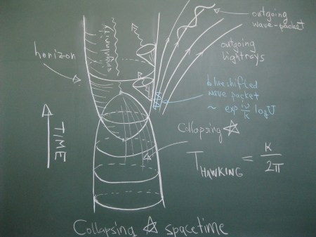
There is also a singularity at the very beginning in the standard Big Bang theory. This again is expected to be a real singularity where the temperature and density become infinite. In this respect the Big Bang can be thought of as a kind of time-reverse of the gravitational collapse that forms a black hole. As was the case with the Schwarzschild solution, many physicists thought that the initial cosmologcal singularity could be a consequence of the special symmetry required by the Cosmological Principle. But this is now known not to be the case. Hawking and Penrose generalized Penrose’s original black hole theorems to show that a singularity invariably exists in the past of an expanding Universe in which certain very general conditions apply.

So is it possible to avoid this singularity? And if so, how?

It is clear that the initial cosmological singularity might well just be a consequence of extrapolating deductions based on the classical ttheory of general relativity into a situation where this theory is no longer valid.  Indeed, Einstein himself wrote:

The theory is based on a separation of the concepts of the gravitational field and matter. While this may be a valid approximation for weak fields, it may presumably be quite inadequate for very high densities of matter. One may not therefore assume the validity of the equations for very high densities and it is just possible that in a unified theory there would be no such singularity.

Einstein, A., 1950. The Meaning of Relativity, 3rd Edition, Princeton University Press.

We need new laws of physics to describe the behaviour of matter in the vicinity of the Big Bang, when the density and temperature are much higher than can be achieved in laboratory experiments. In particular, any theory of matter under such extreme conditions must take account of  quantum effects on a cosmological scale. The name given to the theory of gravity that replaces general relativity at ultra-high energies by taking these effects into account is quantum gravity, but no such theory has yet been constructed.

There are, however, ways of avoiding the initial singularity in classical general relativity without appealing to quantum effects. First, one can propose an equation of state for matter in the very early Universe that does not obey the conditions laid down by Hawking and Penrose. The most important of these conditions is called the strong energy condition: that r+3p/c2>0 where r is the matter density and p is the pressure. There are various ways in which this condition might indeed be violated. In particular, it is violated by a scalar field when its evolution is dominated by its vacuum energy, which is the condition necessary for driving inflationary Universe models into an accelerated expansion.  The vacuum energy of the scalar field may be regarded as an effective cosmological constant; models in which the cosmological constant is included generally have a bounce rather than a singularity: running the clock back, the Universe reaches a minimum size and then expands again.

Whether the singularity is avoidable or not remains an open question, and the issue of whether we can describe the very earliest phases of the Big Bang, before the Planck time, will remain open at least until a complete  theory of quantum gravity is constructed.

Watch “Why the Universe is quite disappointing really – Episode 7” on YouTube

Posted in The Universe and Stuff, YouTube with tags , , , , on September 3, 2020 by telescoper

Back for Episode 7 of this series in which I explain how we can measure the strength of acoustic waves in early Universe using measurements of the cosmic microwave background, and how that leads to the conclusion that the Big Bang wasn’t as loud as you probably thought. You can read more about this here.

The Big Bang Exploded?

Posted in Biographical, The Universe and Stuff with tags , , , on October 15, 2018 by telescoper

I suspect that I’m not the only physicist who receives unsolicited correspondence from people with wacky views on Life, the Universe and Everything. Being a cosmologist, I probably get more of this stuff than those working in less speculative branches of physics. Because I’ve written a few things that appeared in the public domain, I probably even get more than most cosmologists (except the really famous ones of course).

Many “alternative” cosmologists have now discovered email, and indeed the comments box on this blog, but there are still a lot who send their ideas through regular post. Whenever I get a envelope with an address on it that has been typed by an old-fashioned typewriter it’s a dead giveaway that it’s going to be one of those. Sometimes they are just letters (typed or handwritten), but sometimes they are complete manuscripts often with wonderfully batty illustrations. I remember one called Dark Matter, The Great Pyramid and the Theory of Crystal Healing. I used to have an entire filing cabinet filled with things like his, but I took the opportunity of moving from Cardiff some time ago to throw most of them out.

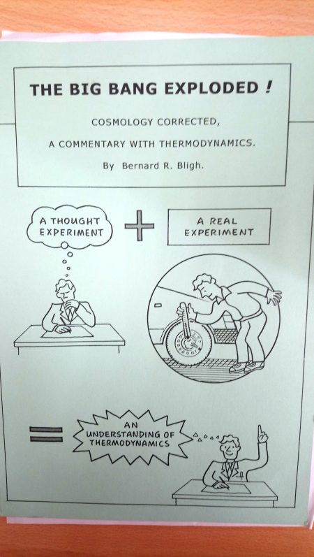
One particular correspondent started writing to me after the publication of my little book, Cosmology: A Very Short Introduction. This chap sent a terse letter to me pointing out that the Big Bang theory was obviously completely wrong. The reason was obvious to anyone who understood thermodynamics. He had spent a lifetime designing high-quality refrigeration equipment and therefore knew what he was talking about (or so he said). He even sent me this booklet about his ideas, which for some reason I have neglected to send for recycling:

His point was that, according to the Big Bang theory, the Universe cools as it expands. Its current temperature is about 3 Kelvin (-270 Celsius or thereabouts) but it is now expanding and cooling. Turning the clock back gives a Universe that was hotter when it was younger. He thought this was all wrong.

The argument is false, my correspondent asserted, because the Universe – by definition – hasn’t got any surroundings and therefore isn’t expanding into anything. Since it isn’t pushing against anything it can’t do any work. The internal energy of the gas must therefore remain constant and since the internal energy of an ideal gas is only a function of its temperature, the expansion of the Universe must therefore be at a constant temperature (i.e. isothermal, rather than adiabatic). He backed up his argument with bona fide experimental results on the free expansion of gases.

I didn’t reply and filed the letter away. Another came, and I did likewise. Increasingly overcome by some form of apoplexy his letters got ruder and ruder, eventually blaming me for the decline of the British education system and demanding that I be fired from my job. Finally, he wrote to the President of the Royal Society demanding that I be “struck off” and forbidden (on grounds of incompetence) ever to teach thermodynamics in a University. The copies of the letters he sent me are still will the pamphlet.

I don’t agree with him that the Big Bang is wrong, but I’ve never had the energy to reply to his rather belligerent letters. However, I think it might be fun to turn this into a little competition, so here’s a challenge for you: provide the clearest and most succint explanation of why the temperature of the expanding Universe does fall with time, despite what my correspondent thought.

Answers via the comment box please!

Cosmology: The Professor’s Old Clothes

Posted in Education, The Universe and Stuff with tags , , , , , , , on January 19, 2018 by telescoper

After spending  a big chunk of yesterday afternoon chatting the cosmic microwave background, yesterday evening I remembered a time when I was trying to explain some of the related concepts to an audience of undergraduate students. As a lecturer you find from time to time that various analogies come to mind that you think will help students understand the physical concepts underpinning what’s going on, and that you hope will complement the way they are developed in a more mathematical language. Sometimes these seem to work well during the lecture, but only afterwards do you find out they didn’t really serve their intended purpose. Sadly it also  sometimes turns out that they can also confuse rather than enlighten…

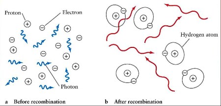
For instance, the two key ideas behind the production of the cosmic microwave background are recombination and the consequent decoupling of matter and radiation. In the early stages of the Big Bang there was a hot plasma consisting mainly of protons and electrons in an intense radiation field. Since it  was extremely hot back then  the plasma was more-or-less  fully ionized, which is to say that the equilibrium for the formation of neutral hydrogen atoms via

p+e^{-} \rightarrow H+ \gamma

lay firmly to the left hand side. The free electrons scatter radiation very efficiently via Compton  scattering

\gamma +e^{-} \rightarrow \gamma + e^{-}

thus establishing thermal equilibrium between the matter and the radiation field. In effect, the plasma is opaque so that the radiation field acquires an accurate black-body spectrum (as observed). As long as the rate of collisions between electrons and photons remains large the radiation temperature adjusts to that of the matter and equilibrium is preserved because matter and radiation are in good thermal contact.


Image credit: James N. Imamura of University of Oregon.

Eventually, however, the temperature falls to a point at which electrons begin to bind with protons to form hydrogen atoms. When this happens the efficiency of scattering falls dramatically and as a consequence the matter and radiation temperatures are no longer coupled together, i.e. decoupling occurs; collisions can longer keep everything in thermal equilibrium. The matter in the Universe then becomes transparent, and the radiation field propagates freely as a kind of relic of the time that it was last in thermal equilibrium. We see that radiation now, heavily redshifted, as the cosmic microwave background.

So far, so good, but I’ve always thought that everyday analogies are useful to explain physics like this so I thought of the following.

When people are young and energetic, they interact very extensively with everyone around them and that process allows them to keep in touch with all the latest trends in clothing, music, books, and so on. As you get older you don’t get about so much , and may even get married (which is just like recombination, not only that it involves the joining together of previously independent entities, but also in the sense that it dramatically  reduces their cross-section for interaction with the outside world).  As time goes on changing trends begin to pass you buy and eventually you become a relic, surrounded by records and books you acquired in the past when you were less introverted, and wearing clothes that went out of fashion years ago.

I’ve used this analogy in the past and students generally find it quite amusing even if it has modest explanatory value. I wasn’t best pleased, however, when a few years ago I set an examination question which asked the students to explain the processes of recombination and decoupling. One answer said

Decoupling explains the state of Prof. Coles’s clothes.

Anyhow, I’m sure there’s more than one reader out there who has had a similar experience with an analogy that wasn’t perhaps as instructive as hoped or which came back to bite you. Feel free to share through the comments box…

What the Power Spectrum misses

Posted in The Universe and Stuff with tags , , , , , , , on August 2, 2017 by telescoper

Just taking a short break from work I chatted over coffee to one of the students here at the Niels Bohr Institute about various things to do with the analysis of signals in the Fourier domain (as you do). That discussion reminded me of this rather old post (from 2009) which I thought might be worth a second airing (after a bit of editing). The discussion is all based on past cosmological data (from WMAP) rather than the most recent (from Planck), but that doesn’t change anything qualitatively. So here you are.

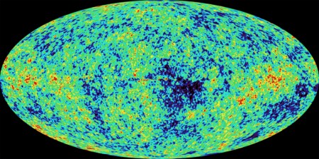
WMapThe picture above shows the all-sky map of fluctuations in the temperature of the cosmic microwave background across the sky as revealed by the Wilkinson Microwave Anisotropy Probe, known to its friends as WMAP.

I spent many long hours fiddling with the data coming from the WMAP experiment, partly because I’ve never quite got over the fact that such wonderful data actually exists. When I started my doctorate in 1985 the whole field of CMB analysis was so much pie in the sky, as no experiments had yet been performed with the sensitivity to reveal the structures we now see. This is because they are very faint and easily buried in noise. The fluctuations in temperature from pixel to pixel across the sky are of order one part in a hundred thousand of the mean temperature (i.e. about 30 microKelvin on a background temperature of about 3 Kelvin). That’s smoother than the surface of a billiard ball. That’s why it took such a long time to make the map shown above, and why it is such a triumphant piece of science.

I blogged a while ago about the idea that the structure we see in this map was produced by sound waves reverberating around the early Universe. The techniques cosmologists use to analyse this sound are similar to those used in branches of acoustics except that we only see things in projection on the celestial sphere which requires a bit of special consideration.

One of the things that sticks in my brain from my undergraduate years is being told that `if you don’t know what you’re doing as a physicist you should start by making a Fourier transform of everything. This approach breaks down the phenomenon being studied into a set of  plane waves with different wavelengths corresponding to analysing the different tones present in a complicated sound.

It’s often very good advice to do such a decomposition for one-dimensional time series or fluctuation fields in three-dimensional Cartesian space, even you do know what you’re doing, but it doesn’t work with a sphere because plane waves don’t fit properly on a curved surface. Fortunately, however, there is a tried-and-tested alternative involving spherical harmonics rather than plane waves.

Spherical harmonics are quite complicated beasts mathematically but they have pretty similar properties to Fourier harmonics in many respects. In particular they are represented as complex numbers having real and imaginary parts or, equivalently, an amplitude and a phase (usually called the argument by mathematicians),

Z=X+iY = R \exp(i\phi)

This latter representation is the most useful one for CMB fluctuations because the simplest versions of inflationary theory predict that the phases φ of each of the spherical harmonic modes should be randomly distributed. What this really means is that there is no information content in their distribution so that the harmonic modes are in a state of maximum statistical disorder or entropy. This property also guarantees that the distribution of fluctuations over the sky should have a Gaussian distribution.

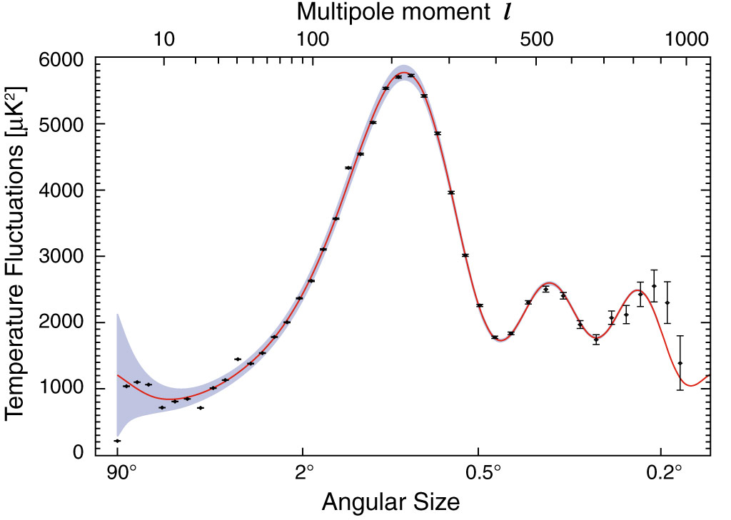
If you accept that the fluctuations are Gaussian then only the amplitudes of the spherical harmonic coefficients are useful. Indeed, their statistical properties can be specified entirely by the variance of these amplitudes as a function of mode frequency. This pre-eminently important function is called the power-spectrum of the fluctuations, and it is shown here for the WMAP data:

080999_powerspectrumm

Although the units on the axes are a bit strange it doesn”t require too much imagination to interpret this in terms of a sound spectrum. There is a characteristic tone (at the position of the big peak) plus a couple of overtones (the bumps at higher frequencies). However these features are not sharp so the overall sound is not at all musical.

If the Gaussian assumption is correct then the power-spectrum contains all the useful statistical information to be gleaned from the CMB sky, which is why so much emphasis has been placed on extracting it accurately from the data.

Conversely, though, the power spectrum is completely insensitive to any information in the distribution of spherical harmonic phases. If something beyond the standard model made the Universe non-Gaussian it would affect the phases of the harmonic modes in a way that would make them non-random.

However,I will now show you how important phase information could actually be, if only we could find a good way of exploiting it. Let’s start with a map of the Earth, with the colour representing height of the surface above mean sea level:

sw_world

You can see the major mountain ranges (Andes, Himalayas) quite clearly as red in this picture and note how high Antarctica is…that’s one of the reasons so much astronomy is done there.

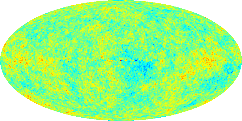
Now, using the same colour scale we have the WMAP data again (in Galactic coordinates).

sw_ilc

The virture of this representation of the map is that it shows how smooth the microwave sky is compared to the surface of the Earth. Note also that you can see a bit of crud in the plane of the Milky Way that serves as a reminder of the difficulty of cleaning the foregrounds out.

Clearly these two maps have completely different power spectra. The Earth is dominated by large features made from long-wavelength modes whereas the CMB sky has relatively more small-scale fuzz.

Now I’m going to play with these maps in the following rather peculiar way. First, I make a spherical harmonic transform of each of them. This gives me two sets of complex numbers, one for the Earth and one for WMAP. Following the usual fashion, I think of these as two sets of amplitudes and two sets of phases. Note that the spherical harmonic transformation preserves all the information in the sky maps, it’s just a different representation.

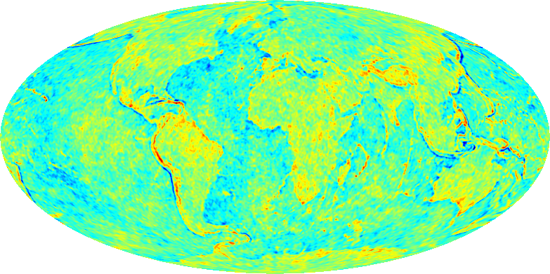
Now what I do is swap the amplitudes and phases for the two maps. First, I take the amplitudes of WMAP and put them with the phases for the Earth. That gives me the spherical harmonic representation of a new data set which I can reveal by doing an inverse spherical transform:

sw_worldphases

This map has exactly the same amplitudes for each mode as the WMAP data and therefore possesses an identical power spectrum to that shown above. Clearly, though, this particular CMB sky is not compatible with the standard cosmological model! Notice that all the strongly localised features such as coastlines appear by virtue of information contained in the phases but absent from the power-spectrum.

To understand this think how sharp features appear in a Fourier transform. A sharp spike at a specific location actually produces a broad spectrum of Fourier modes with different frequencies. These modes have to add in coherently at the location of the spike and cancel out everywhere else, so their phases are strongly correlated. A sea of white noise also has a flat power spectrum but has random phases. The key difference between these two configurations is not revealed by their spectra but by their phases.

Fortunately there is nothing quite as wacky as a picture of the Earth in the real data, but it makes the point that there are more things in Heaven and Earth than can be described in terms of the power spectrum!

Finally, perhaps in your mind’s eye you might consider what it might look lie to do the reverse experiment: recombine the phases of WMAP with the amplitudes of the Earth.

sw_ilcphases

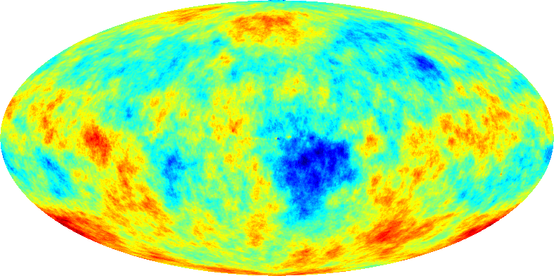
If the WMAP data are actually Gaussian, then this map is a sort of random-phase realisation of the Earth’s power spectrum. Alternatively you can see that it is the result of running a kind of weird low-pass filter over the WMAP fluctuations. The only striking things it reveals are (i) a big blue hole associated with foreground contamination, (ii) a suspicious excess of red in the galactic plane owing to the same problem, and (iiI) a strong North-South asymmetry arising from the presence of Antarctica.

There’s no great scientific result here, just a proof that spherical harmonic phases are potentially interesting because of the information they contain about strongly localised features

PS. These pictures were made by a former PhD student of mine, Patrick Dineen, who has since quit astrophysics  to work in the financial sector for Winton Capital, which has over the years recruited a number of astronomy and cosmology graduates and also sponsors a Royal Astronomical Society prize. That shows that the skills and knowledge obtained in the seemingly obscure field of cosmological data analysis have applications elsewhere!


A Quite Interesting Question: How Loud Was the Big Bang?

Posted in The Universe and Stuff with tags , , , , , , , on March 16, 2017 by telescoper

I just found out this morning that this blog got a mention on the QI Podcast. It’s taken a while for this news to reach me, as the item concerned is two years old! You can find this discussion here, about 16 minutes in. And no, it’s not in connection with yawning psychopaths. It was about the vexed question of how loud was the Big Bang?

I’ve posted on this before (here and here)but since I’m very busy again today I  should recycle the discussion, and update it as it relates to the cosmic microwave background, which is what one of the things I work on on the rare occasions on which I get to do anything interesting.

As you probably know the Big Bang theory involves the assumption that the entire Universe – not only the matter and energy but also space-time itself – had its origins in a single event a finite time in the past and it has been expanding ever since. The earliest mathematical models of what we now call the  Big Bang were derived independently by Alexander Friedman and George Lemaître in the 1920s. The term “Big Bang” was later coined by Fred Hoyle as a derogatory description of an idea he couldn’t stomach, but the phrase caught on. Strictly speaking, though, the Big Bang was a misnomer.

Friedman and Lemaître had made mathematical models of universes that obeyed the Cosmological Principle, i.e. in which the matter was distributed in a completely uniform manner throughout space. Sound consists of oscillating fluctuations in the pressure and density of the medium through which it travels. These are longitudinal “acoustic” waves that involve successive compressions and rarefactions of matter, in other words departures from the purely homogeneous state required by the Cosmological Principle. The Friedman-Lemaitre models contained no sound waves so they did not really describe a Big Bang at all, let alone how loud it was.

However, as I have blogged about before, newer versions of the Big Bang theory do contain a mechanism for generating sound waves in the early Universe and, even more importantly, these waves have now been detected and their properties measured.

Planck_CMB

The above image shows the variations in temperature of the cosmic microwave background as charted by the Planck Satellite. The average temperature of the sky is about 2.73 K but there are variations across the sky that have an rms value of about 0.08 milliKelvin. This corresponds to a fractional variation of a few parts in a hundred thousand relative to the mean temperature. It doesn’t sound like much, but this is evidence for the existence of primordial acoustic waves and therefore of a Big Bang with a genuine “Bang” to it.

A full description of what causes these temperature fluctuations would be very complicated but, roughly speaking, the variation in temperature you corresponds directly to variations in density and pressure arising from sound waves.

So how loud was it?

The waves we are dealing with have wavelengths up to about 200,000 light years and the human ear can only actually hear sound waves with wavelengths up to about 17 metres. In any case the Universe was far too hot and dense for there to have been anyone around listening to the cacophony at the time. In some sense, therefore, it wouldn’t have been loud at all because our ears can’t have heard anything.

Setting aside these rather pedantic objections – I’m never one to allow dull realism to get in the way of a good story- we can get a reasonable value for the loudness in terms of the familiar language of decibels. This defines the level of sound (L) logarithmically in terms of the rms pressure level of the sound wave Prms relative to some reference pressure level Pref

L=20 log10[Prms/Pref].

(the 20 appears because of the fact that the energy carried goes as the square of the amplitude of the wave; in terms of energy there would be a factor 10).

There is no absolute scale for loudness because this expression involves the specification of the reference pressure. We have to set this level by analogy with everyday experience. For sound waves in air this is taken to be about 20 microPascals, or about 2×10⁻¹⁰ times the ambient atmospheric air pressure which is about 100,000 Pa.  This reference is chosen because the limit of audibility for most people corresponds to pressure variations of this order and these consequently have L=0 dB. It seems reasonable to set the reference pressure of the early Universe to be about the same fraction of the ambient pressure then, i.e.

Pref~2×10⁻¹⁰ Pamb.

The physics of how primordial variations in pressure translate into observed fluctuations in the CMB temperature is quite complicated, because the primordial universe consists of a plasma rather than air. Moreover, the actual sound of the Big Bang contains a mixture of wavelengths with slightly different amplitudes. In fact here is the spectrum, showing a distinctive signature that looks, at least in this representation, like a fundamental tone and a series of harmonics…

Planck_power_spectrum_orig


If you take into account all this structure it all gets a bit messy, but it’s quite easy to get a rough but reasonable estimate by ignoring all these complications. We simply take the rms pressure variation to be the same fraction of ambient pressure as the averaged temperature variation are compared to the average CMB temperature,  i.e.

Prms~ a few ×10-5Pamb.

If we do this, scaling both pressures in logarithm in the equation in proportion to the ambient pressure, the ambient pressure cancels out in the ratio, which turns out to be a few times 10-5. With our definition of the decibel level we find that waves of this amplitude, i.e. corresponding to variations of one part in a hundred thousand of the reference level, give roughly L=100dB while part in ten thousand gives about L=120dB. The sound of the Big Bang therefore peaks at levels just a bit less than 120 dB.

cooler_decibel_chart

As you can see in the Figure above, this is close to the threshold of pain,  but it’s perhaps not as loud as you might have guessed in response to the initial question. Modern popular beat combos often play their dreadful rock music much louder than the Big Bang….

A useful yardstick is the amplitude  at which the fluctuations in pressure are comparable to the mean pressure. This would give a factor of about 1010 in the logarithm and is pretty much the limit that sound waves can propagate without distortion. These would have L≈190 dB. It is estimated that the 1883 Krakatoa eruption produced a sound level of about 180 dB at a range of 100 miles. The QI podcast also mentions  that blue whales make a noise that corresponds to about 188 decibels. By comparison the Big Bang was little more than a whimper..

PS. If you would like to read more about the actual sound of the Big Bang, have a look at John Cramer’s webpages. You can also download simulations of the actual sound. If you listen to them you will hear that it’s more of  a “Roar” than a “Bang” because the sound waves don’t actually originate at a single well-defined event but are excited incoherently all over the Universe.

Life as a Condition of Cosmology

Posted in The Universe and Stuff with tags , , , , , , , on November 7, 2015 by telescoper

Trigger Warnings: Bayesian Probability and the Anthropic Principle!

Once upon a time I was involved in setting up a cosmology conference in Valencia (Spain). The principal advantage of being among the organizers of such a meeting is that you get to invite yourself to give a talk and to choose the topic. On this particular occasion, I deliberately abused my privilege and put myself on the programme to talk about the “Anthropic Principle”. I doubt if there is any subject more likely to polarize a scientific audience than this. About half the participants present in the meeting stayed for my talk. The other half ran screaming from the room. Hence the trigger warnings on this post. Anyway, I noticed a tweet this morning from Jon Butterworth advertising a new blog post of his on the very same subject so I thought I’d while away a rainy November afternoon with a contribution of my own.

In case you weren’t already aware, the Anthropic Principle is the name given to a class of ideas arising from the suggestion that there is some connection between the material properties of the Universe as a whole and the presence of human life within it. The name was coined by Brandon Carter in 1974 as a corrective to the “Copernican Principle” that man does not occupy a special place in the Universe. A naïve application of this latter principle to cosmology might lead us to think that we could have evolved in any of the myriad possible Universes described by the system of Friedmann equations. The Anthropic Principle denies this, because life could not have evolved in all possible versions of the Big Bang model. There are however many different versions of this basic idea that have different logical structures and indeed different degrees of credibility. It is not really surprising to me that there is such a controversy about this particular issue, given that so few physicists and astronomers take time to study the logical structure of the subject, and this is the only way to assess the meaning and explanatory value of propositions like the Anthropic Principle. My former PhD supervisor, John Barrow (who is quoted in John Butterworth’s post) wrote the definite text on this topic together with Frank Tipler to which I refer you for more background. What I want to do here is to unpick this idea from a very specific perspective and show how it can be understood quite straightfowardly in terms of Bayesian reasoning. I’ll begin by outlining this form of inferential logic.

I’ll start with Bayes’ theorem which for three logical propositions (such as statements about the values of parameters in theory) A, B and C can be written in the form

P(B|AC) = K^{-1}P(B|C)P(A|BC) = K^{-1} P(AB|C)

where

K=P(A|C).

This is (or should be!)  uncontroversial as it is simply a result of the sum and product rules for combining probabilities. Notice, however, that I’ve not restricted it to two propositions A and B as is often done, but carried throughout an extra one (C). This is to emphasize the fact that, to a Bayesian, all probabilities are conditional on something; usually, in the context of data analysis this is a background theory that furnishes the framework within which measurements are interpreted. If you say this makes everything model-dependent, then I’d agree. But every interpretation of data in terms of parameters of a model is dependent on the model. It has to be. If you think it can be otherwise then I think you’re misguided.

In the equation,  P(B|C) is the probability of B being true, given that C is true . The information C need not be definitely known, but perhaps assumed for the sake of argument. The left-hand side of Bayes’ theorem denotes the probability of B given both A and C, and so on. The presence of C has not changed anything, but is just there as a reminder that it all depends on what is being assumed in the background. The equation states  a theorem that can be proved to be mathematically correct so it is – or should be – uncontroversial.

To a Bayesian, the entities A, B and C are logical propositions which can only be either true or false. The entities themselves are not blurred out, but we may have insufficient information to decide which of the two possibilities is correct. In this interpretation, P(A|C) represents the degree of belief that it is consistent to hold in the truth of A given the information C. Probability is therefore a generalization of the “normal” deductive logic expressed by Boolean algebra: the value “0” is associated with a proposition which is false and “1” denotes one that is true. Probability theory extends  this logic to the intermediate case where there is insufficient information to be certain about the status of the proposition.

A common objection to Bayesian probability is that it is somehow arbitrary or ill-defined. “Subjective” is the word that is often bandied about. This is only fair to the extent that different individuals may have access to different information and therefore assign different probabilities. Given different information C and C′ the probabilities P(A|C) and P(A|C′) will be different. On the other hand, the same precise rules for assigning and manipulating probabilities apply as before. Identical results should therefore be obtained whether these are applied by any person, or even a robot, so that part isn’t subjective at all.

In fact I’d go further. I think one of the great strengths of the Bayesian interpretation is precisely that it does depend on what information is assumed. This means that such information has to be stated explicitly. The essential assumptions behind a result can be – and, regrettably, often are – hidden in frequentist analyses. Being a Bayesian forces you to put all your cards on the table.

To a Bayesian, probabilities are always conditional on other assumed truths. There is no such thing as an absolute probability, hence my alteration of the form of Bayes’s theorem to represent this. A probability such as P(A) has no meaning to a Bayesian: there is always conditioning information. For example, if  I blithely assign a probability of 1/6 to each face of a dice, that assignment is actually conditional on me having no information to discriminate between the appearance of the faces, and no knowledge of the rolling trajectory that would allow me to make a prediction of its eventual resting position.

In tbe Bayesian framework, probability theory  becomes not a branch of experimental science but a branch of logic. Like any branch of mathematics it cannot be tested by experiment but only by the requirement that it be internally self-consistent. This brings me to what I think is one of the most important results of twentieth century mathematics, but which is unfortunately almost unknown in the scientific community. In 1946, Richard Cox derived the unique generalization of Boolean algebra under the assumption that such a logic must involve associated a single number with any logical proposition. The result he got is beautiful and anyone with any interest in science should make a point of reading his elegant argument. It turns out that the only way to construct a consistent logic of uncertainty incorporating this principle is by using the standard laws of probability. There is no other way to reason consistently in the face of uncertainty than probability theory. Accordingly, probability theory always applies when there is insufficient knowledge for deductive certainty. Probability is inductive logic.

This is not just a nice mathematical property. This kind of probability lies at the foundations of a consistent methodological framework that not only encapsulates many common-sense notions about how science works, but also puts at least some aspects of scientific reasoning on a rigorous quantitative footing. This is an important weapon that should be used more often in the battle against the creeping irrationalism one finds in society at large.

To see how the Bayesian approach provides a methodology for science, let us consider a simple example. Suppose we have a hypothesis H (some theoretical idea that we think might explain some experiment or observation). We also have access to some data D, and we also adopt some prior information I (which might be the results of other experiments and observations, or other working assumptions). What we want to know is how strongly the data D supports the hypothesis H given my background assumptions I. To keep it easy, we assume that the choice is between whether H is true or H is false. In the latter case, “not-H” or H′ (for short) is true. If our experiment is at all useful we can construct P(D|HI), the probability that the experiment would produce the data set D if both our hypothesis and the conditional information are true.

The probability P(D|HI) is called the likelihood; to construct it we need to have   some knowledge of the statistical errors produced by our measurement. Using Bayes’ theorem we can “invert” this likelihood to give P(H|DI), the probability that our hypothesis is true given the data and our assumptions. The result looks just like we had in the first two equations:

P(H|DI) = K^{-1}P(H|I)P(D|HI) .

Now we can expand the “normalising constant” K because we know that either H or H′ must be true. Thus

K=P(D|I)=P(H|I)P(D|HI)+P(H^{\prime}|I) P(D|H^{\prime}I)

The P(H|DI) on the left-hand side of the first expression is called the posterior probability; the right-hand side involves P(H|I), which is called the prior probability and the likelihood P(D|HI). The principal controversy surrounding Bayesian inductive reasoning involves the prior and how to define it, which is something I’ll comment on in a future post.

The Bayesian recipe for testing a hypothesis assigns a large posterior probability to a hypothesis for which the product of the prior probability and the likelihood is large. It can be generalized to the case where we want to pick the best of a set of competing hypothesis, say H1 …. Hn. Note that this need not be the set of all possible hypotheses, just those that we have thought about. We can only choose from what is available. The hypothesis may be relatively simple, such as that some particular parameter takes the value x, or they may be composite involving many parameters and/or assumptions. For instance, the Big Bang model of our universe is a very complicated hypothesis, or in fact a combination of hypotheses joined together,  involving at least a dozen parameters which can’t be predicted a priori but which have to be estimated from observations.

The required result for multiple hypotheses is pretty straightforward: the sum of the two alternatives involved in K above simply becomes a sum over all possible hypotheses, so that

P(H_i|DI) = K^{-1}P(H_i|I)P(D|H_iI),

and

K=P(D|I)=\sum P(H_j|I)P(D|H_jI)

If the hypothesis concerns the value of a parameter – in cosmology this might be, e.g., the mean density of the Universe expressed by the density parameter Ω0 – then the allowed space of possibilities is continuous. The sum in the denominator should then be replaced by an integral, but conceptually nothing changes. Our “best” hypothesis is the one that has the greatest posterior probability.

From a frequentist stance the procedure is often instead to just maximize the likelihood. According to this approach the best theory is the one that makes the data most probable. This can be the same as the most probable theory, but only if the prior probability is constant, but the probability of a model given the data is generally not the same as the probability of the data given the model. I’m amazed how many practising scientists make this error on a regular basis.

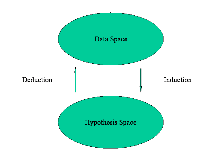
The following figure might serve to illustrate the difference between the frequentist and Bayesian approaches. In the former case, everything is done in “data space” using likelihoods, and in the other we work throughout with probabilities of hypotheses, i.e. we think in hypothesis space. I find it interesting to note that most theorists that I know who work in cosmology are Bayesians and most observers are frequentists!

As I mentioned above, it is the presence of the prior probability in the general formula that is the most controversial aspect of the Bayesian approach. The attitude of frequentists is often that this prior information is completely arbitrary or at least “model-dependent”. Being empirically-minded people, by and large, they prefer to think that measurements can be made and interpreted without reference to theory at all.

Assuming we can assign the prior probabilities in an appropriate way what emerges from the Bayesian framework is a consistent methodology for scientific progress. The scheme starts with the hardest part – theory creation. This requires human intervention, since we have no automatic procedure for dreaming up hypothesis from thin air. Once we have a set of hypotheses, we need data against which theories can be compared using their relative probabilities. The experimental testing of a theory can happen in many stages: the posterior probability obtained after one experiment can be fed in, as prior, into the next. The order of experiments does not matter. This all happens in an endless loop, as models are tested and refined by confrontation with experimental discoveries, and are forced to compete with new theoretical ideas. Often one particular theory emerges as most probable for a while, such as in particle physics where a “standard model” has been in existence for many years. But this does not make it absolutely right; it is just the best bet amongst the alternatives. Likewise, the Big Bang model does not represent the absolute truth, but is just the best available model in the face of the manifold relevant observations we now have concerning the Universe’s origin and evolution. The crucial point about this methodology is that it is inherently inductive: all the reasoning is carried out in “hypothesis space” rather than “observation space”.  The primary form of logic involved is not deduction but induction. Science is all about inverse reasoning.

Now, back to the anthropic principle. The point is that we can observe that life exists in our Universe and this observation must be incorporated as conditioning information whenever we try to make inferences about cosmological models if we are to reason consistently. In other words, the existence of life is a datum that must be incorporated in the conditioning information I mentioned above.

Suppose we have a model of the Universe M that contains various parameters which can be fixed by some form of observation. Let U be the proposition that these parameters take specific values U1, U2, and so on. Anthropic arguments revolve around the existence of life, so let L be the proposition that intelligent life evolves in the Universe. Note that the word “anthropic” implies specifically human life, but many versions of the argument do not necessarily accommodate anything more complicated than a virus.

Using Bayes’ theorem we can write

P(U|L,M)=K^{-1} P(U|M)P(L|U,M)

The dependence of the posterior probability P(U|L,M) on the likelihood P(L|U,M) demonstrates that the values of U for which P(L|U,M) is larger correspond to larger values of P(U|L,M); K is just a normalizing constant for the purpose of this argument. Since life is observed in our Universe the model-parameters which make life more probable must be preferred to those that make it less so. To go any further we need to say something about the likelihood and the prior. Here the complexity and scope of the model makes it virtually impossible to apply in detail the symmetry principles usually exploited to define priors for physical models. On the other hand, it seems reasonable to assume that the prior is broad rather than sharply peaked; if our prior knowledge of which universes are possible were so definite then we wouldn’t really be interested in knowing what observations could tell us. If now the likelihood is sharply peaked in U then this will be projected directly into the posterior distribution.

We have to assign the likelihood using our knowledge of how galaxies, stars and planets form, how planets are distributed in orbits around stars, what conditions are needed for life to evolve, and so on. There are certainly many gaps in this knowledge. Nevertheless if any one of the steps in this chain of knowledge requires very finely-tuned parameter choices then we can marginalize over the remaining steps and still end up with a sharp peak in the remaining likelihood and so also in the posterior probability. For example, there are plausible reasons for thinking that intelligent life has to be carbon-based, and therefore evolve on a planet. It is reasonable to infer, therefore, that P(U|L,M) should prefer some values of U. This means that there is a correlation between the propositions U and L in the sense that knowledge of one should, through Bayesian reasoning, enable us to make inferences about the other.

It is very difficult to make this kind of argument rigorously quantitative, but I can illustrate how the argument works with a simplified example. Let us suppose that the relevant parameters contained in the set U include such quantities as Newton’s gravitational constant G, the charge on the electron e, and the mass of the proton m. These are usually termed fundamental constants. The argument above indicates that there might be a connection between the existence of life and the value that these constants jointly take. Moreover, there is no reason why this kind of argument should not be used to find the values of fundamental constants in advance of their measurement. The ordering of experiment and theory is merely an historical accident; the process is cyclical. An illustration of this type of logic is furnished by the case of a plant whose seeds germinate only after prolonged rain. A newly-germinated (and intelligent) specimen could either observe dampness in the soil directly, or infer it using its own knowledge coupled with the observation of its own germination. This type, used properly, can be predictive and explanatory.

This argument is just one example of a number of its type, and it has clear (but limited) explanatory power. Indeed it represents a fruitful application of Bayesian reasoning. The question is how surprised we should be that the constants of nature are observed to have their particular values? That clearly requires a probability based answer. The smaller the probability of a specific joint set of values (given our prior knowledge) then the more surprised we should be to find them. But this surprise should be bounded in some way: the values have to lie somewhere in the space of possibilities. Our argument has not explained why life exists or even why the parameters take their values but it has elucidated the connection between two propositions. In doing so it has reduced the number of unexplained phenomena from two to one. But it still takes our existence as a starting point rather than trying to explain it from first principles.

Arguments of this type have been called Weak Anthropic Principle by Brandon Carter and I do not believe there is any reason for them to be at all controversial. They are simply Bayesian arguments that treat the existence of life as an observation about the Universe that is treated in Bayes’ theorem in the same way as all other relevant data and whatever other conditioning information we have. If more scientists knew about the inductive nature of their subject, then this type of logic would not have acquired the suspicious status that it currently has.

A Galaxy at Record Redshift?

Posted in The Universe and Stuff with tags , , , , , on July 13, 2015 by telescoper

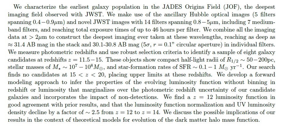
Skimming through the arXiv this morning I discovered a paper by Zitrin et al. with the following abstract:


abstract_z

I’m not sure if the figures are all significant, but a redshift of z=8.68 makes this the most distant spectroscopically confirmed galaxy on record with a present proper distance of about 9.3 Gpc according to the standard cosmological model, just pipping the previous record holder (whose redshift was in any case disputed). Light from this galaxy has taken about 13.1 Gyr to reach us; that means light set out from it when the Universe was only about 4% of its current age, only about 600 million years after the Big Bang. (Those figures were obtained using the inestimable Ned Wright’s cosmology calculator.)

We are presumably seeing a very young object, in which stars are forming at a considerable rate to account for its brightness. We don’t know exactly when the first stars formed and began to ionize the intergalactic medium, but every time the cosmic distance record is broken we push that time back closer to the Big Bang.

Mind you, I can’t say I’m overwhelmingly convinced by the identification of the redshifted Lyman-α line:

high_zBut what do I know? I’m a theorist whose suspicious of data. Any observers care to comment?

Why the Big Bang wasn’t as loud as you think…

Posted in The Universe and Stuff with tags , , , , , on March 31, 2015 by telescoper

So how loud was the Big Bang?

I’ve posted on this before but a comment posted today reminded me that perhaps I should recycle it and update it as it relates to the cosmic microwave background, which is what I work on on the rare occasions on which I get to do anything interesting.

As you probably know the Big Bang theory involves the assumption that the entire Universe – not only the matter and energy but also space-time itself – had its origins in a single event a finite time in the past and it has been expanding ever since. The earliest mathematical models of what we now call the  Big Bang were derived independently by Alexander Friedman and George Lemaître in the 1920s. The term “Big Bang” was later coined by Fred Hoyle as a derogatory description of an idea he couldn’t stomach, but the phrase caught on. Strictly speaking, though, the Big Bang was a misnomer.

Friedman and Lemaître had made mathematical models of universes that obeyed the Cosmological Principle, i.e. in which the matter was distributed in a completely uniform manner throughout space. Sound consists of oscillating fluctuations in the pressure and density of the medium through which it travels. These are longitudinal “acoustic” waves that involve successive compressions and rarefactions of matter, in other words departures from the purely homogeneous state required by the Cosmological Principle. The Friedman-Lemaitre models contained no sound waves so they did not really describe a Big Bang at all, let alone how loud it was.

However, as I have blogged about before, newer versions of the Big Bang theory do contain a mechanism for generating sound waves in the early Universe and, even more importantly, these waves have now been detected and their properties measured.

Planck_CMB

The above image shows the variations in temperature of the cosmic microwave background as charted by the Planck Satellite. The average temperature of the sky is about 2.73 K but there are variations across the sky that have an rms value of about 0.08 milliKelvin. This corresponds to a fractional variation of a few parts in a hundred thousand relative to the mean temperature. It doesn’t sound like much, but this is evidence for the existence of primordial acoustic waves and therefore of a Big Bang with a genuine “Bang” to it.

A full description of what causes these temperature fluctuations would be very complicated but, roughly speaking, the variation in temperature you corresponds directly to variations in density and pressure arising from sound waves.

So how loud was it?

The waves we are dealing with have wavelengths up to about 200,000 light years and the human ear can only actually hear sound waves with wavelengths up to about 17 metres. In any case the Universe was far too hot and dense for there to have been anyone around listening to the cacophony at the time. In some sense, therefore, it wouldn’t have been loud at all because our ears can’t have heard anything.

Setting aside these rather pedantic objections – I’m never one to allow dull realism to get in the way of a good story- we can get a reasonable value for the loudness in terms of the familiar language of decibels. This defines the level of sound (L) logarithmically in terms of the rms pressure level of the sound wave Prms relative to some reference pressure level Pref

L=20 log10[Prms/Pref].

(the 20 appears because of the fact that the energy carried goes as the square of the amplitude of the wave; in terms of energy there would be a factor 10).

There is no absolute scale for loudness because this expression involves the specification of the reference pressure. We have to set this level by analogy with everyday experience. For sound waves in air this is taken to be about 20 microPascals, or about 2×10⁻¹⁰ times the ambient atmospheric air pressure which is about 100,000 Pa.  This reference is chosen because the limit of audibility for most people corresponds to pressure variations of this order and these consequently have L=0 dB. It seems reasonable to set the reference pressure of the early Universe to be about the same fraction of the ambient pressure then, i.e.

Pref~2×10⁻¹⁰ Pamb.

The physics of how primordial variations in pressure translate into observed fluctuations in the CMB temperature is quite complicated, because the primordial universe consists of a plasma rather than air. Moreover, the actual sound of the Big Bang contains a mixture of wavelengths with slightly different amplitudes. In fact here is the spectrum, showing a distinctive signature that looks, at least in this representation, like a fundamental tone and a series of harmonics…

Planck_power_spectrum_orig


If you take into account all this structure it all gets a bit messy, but it’s quite easy to get a rough but reasonable estimate by ignoring all these complications. We simply take the rms pressure variation to be the same fraction of ambient pressure as the averaged temperature variation are compared to the average CMB temperature,  i.e.

Prms~ a few ×10-5Pamb.

If we do this, scaling both pressures in logarithm in the equation in proportion to the ambient pressure, the ambient pressure cancels out in the ratio, which turns out to be a few times 10-5. With our definition of the decibel level we find that waves of this amplitude, i.e. corresponding to variations of one part in a hundred thousand of the reference level, give roughly L=100dB while part in ten thousand gives about L=120dB. The sound of the Big Bang therefore peaks at levels just a bit less than 120 dB.

cooler_decibel_chart

As you can see in the Figure above, this is close to the threshold of pain,  but it’s perhaps not as loud as you might have guessed in response to the initial question. Modern popular beat combos often play their dreadful rock music much louder than the Big Bang….

A useful yardstick is the amplitude  at which the fluctuations in pressure are comparable to the mean pressure. This would give a factor of about 1010 in the logarithm and is pretty much the limit that sound waves can propagate without distortion. These would have L≈190 dB. It is estimated that the 1883 Krakatoa eruption produced a sound level of about 180 dB at a range of 100 miles. By comparison the Big Bang was little more than a whimper.

PS. If you would like to read more about the actual sound of the Big Bang, have a look at John Cramer’s webpages. You can also download simulations of the actual sound. If you listen to them you will hear that it’s more of  a “Roar” than a “Bang” because the sound waves don’t actually originate at a single well-defined event but are excited incoherently all over the Universe.