During March 2014 this blog received the most traffic it has ever had (reaching almost 10,000 hits per day at one point). The reason for that was the announcement of the “discovery” of primordial gravitational waves by the BICEP2 experiment. Despite all the hype at the time I wasn’t convinced. This is what I said in an interview with Physics World:
It seems to me though that there’s a significant possibility of some of the polarization signal in E and B [modes] not being cosmological. This is a very interesting result, but I’d prefer to reserve judgement until it is confirmed by other experiments. If it is genuine, then the spectrum is a bit strange and may indicate something added to the normal inflationary recipe.
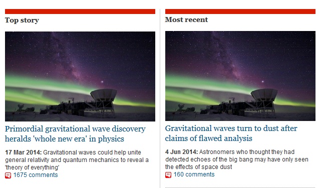
I also blogged about this several times, e.g. here. It turns out I was right to be unconvinced as the signal detected by BICEP2 was dominated by polarized foreground emission. The story is summarized by these two news stories just a few months apart:
Anyway, the search for primordial gravitational waves continues. The latest publication on this topic came out earlier this month in Physical Review Letters and you can also find it on the arXiv here. The last sentence of the abstract is:
These are the strongest constraints to date on primordial gravitational waves.
In other words, seven years on from the claimed “discovery” there is still no evidence for anything but polarized dust emission…
I have been struck by the number of people upset by the latest analysis of SARS-Cov-2 “variants of concern” byPublic Health England. In particular it is in the report that over 40% of those dying from the so-called Delta Variant have had both vaccine jabs. I even saw some comments on social media from people saying that this proves that the vaccines are useless against this variant and as a consequence they weren’t going to bother getting their second jab.
This is dangerous nonsense and I think it stems – as much dangerous nonsense does – from a misunderstanding of basic probability which comes up in a number of situations, including the Prosecutor’s Fallacy. I’ll try to clarify it here with a bit of probability theory. The same logic as the following applies if you specify serious illness or mortality, but I’ll keep it simple by just talking about contracting Covid-19. When I write about probabilities you can think of these as proportions within the population so I’ll use the terms probability and proportion interchangeably in the following.
Denote by P[C|V] the conditional probability that a fully vaccinated person becomes ill from Covid-19. That is considerably smaller than P[C| not V] (by a factor of ten or so given the efficacy of the vaccines). Vaccines do not however deliver perfect immunity so P[C|V]≠0.
Let P[V|C] be the conditional probability of a person with Covid-19 having been fully vaccinated. Or, if you prefer, the proportion of people with Covid-19 who are fully vaccinated..
Now the first thing to point out is that these conditional probability are emphatically not equal. The probability of a female person being pregnant is not the same as the probability of a pregnant person being female.
We can find the relationship between P[C|V] and P[V|C] using the joint probability P[V,C]=P[V,C] of a person having been fully vaccinated and contracting Covid-19. This can be decomposed in two ways: P[V,C]=P[V]P[C|V]=P[C]P[V|C]=P[V,C], where P[V] is the proportion of people fully vaccinated and P[C] is the proportion of people who have contracted Covid-19. This gives P[V|C]=P[V]P[C|V]/P[C].
This result is nothing more than the famous Bayes Theorem.
Now P[C] is difficult to know exactly because of variable testing rates and other selection effects but is presumably quite small. The total number of positive tests since the pandemic began in the UK is about 5M which is less than 10% of the population. The proportion of the population fully vaccinated on the other hand is known to be about 50% in the UK. We can be pretty sure therefore that P[V]»P[C]. This in turn means that P[V|C]»P[C|V].
In words this means that there is nothing to be surprised about in the fact that the proportion of people being infected with Covid-19 is significantly larger than the probability of a vaccinated person catching Covid-19. It is expected that the majority of people catching Covid-19 in the current phase of the pandemic will have been fully vaccinated.
(As a commenter below points out, in the limit when everyone has been vaccinated 100% of the people who catch Covid-19 will have been vaccinated. The point is that the number of people getting ill and dying will be lower than in an unvaccinated population.)
The proportion of those dying of Covid-19 who have been fully vaccinated will also be high, a point also made here.
It’s difficult to be quantitatively accurate here because there are other factors involved in the risk of becoming ill with Covid-19, chiefly age. The reason this poses a problem is that in my countries vaccinations have been given preferentially to those deemed to be at high risk. Younger people are at relatively low risk of serious illness or death from Covid-19 whether or not they are vaccinated compared to older people, but the latter are also more likely to have been vaccinated. To factor this into the calculation above requires an additional piece of conditioning information. We could express this crudely in terms of a binary condition High Risk (H) or Low Risk (L) and construct P(V|L,H) etc but I don’t have the time or information to do this.
So please don’t be taken in by this fallacy. Vaccines do work. Get your second jab (or your first if you haven’t done it yet). It might save your life.
The other day, via Twitter, I came across an interesting blog post about the relatively recent resurgence of Bayesian reasoning in science. That piece had triggered a discussion about why cosmologists seem to be largely Bayesian in outlook, so I thought I’d share a few thoughts about that. You can find a lot of posts about various aspects of Bayesian reasoning on this blog, e.g. here.
When I was an undergraduate student I didn’t think very much about statistics at all, so when I started my DPhil studies I realized I had a great deal to learn. However, at least to start with, I mainly used frequentist methods. Looking back I think that’s probably because I was working on cosmic microwave background statistics and we didn’t really have any data back in 1985. Or actually we had data, but no firm detections. I was therefore taking models and calculating things in what I would call the forward direction, indicated by the up arrow. What I was trying to do was find statistical descriptors that looked likely to be able to discriminate between different models but I didn’t have the data.
Once measurements started to become available the inverse-reasoning part of the diagram indicated by the downward arrow came to the fore. It was only then that it started to become necessary to make firm statements about which models were favoured by the data and which weren’t. That is what Bayesian methods do best, especially when you have to combine different data sets.
By the early 1990s I was pretty much a confirmed Bayesian – as were quite a few fellow theorists -but I noticed that most observational cosmologists I knew were confirmed frequentists. I put that down to the fact that they preferred to think in “measurement space” rather than “theory space”, the latter requiring the inductive step furnished by Bayesian reasoning indicated by the downward arrow. As cosmology has evolved the separation between theorists and observers in some areas – especially CMB studies – has all but vanished and there’s a huge activity at the interface between theory and measurement.
But my first exposure to Bayesian reasoning came long before that change. I wasn’t aware of its usefulness until 1987, when I returned to Cambridge for a conference called The Post-Recombination Universe organized by Nick Kaiser and Anthony Lasenby. There was an interesting discussion in one session about how to properly state the upper limit on CMB fluctuations arising from a particular experiment, which had been given incorrectly in a paper using a frequentist argument. During the discussion, Nick described Anthony as a “Born-again Bayesian”, a phrase that stuck in my memory though I’m still not sure whether or not it was meant as an insult.
It may be the case for many people that a relatively simple example convinces them of the superiority of a particular method or approach. I had previously found statistical methods – especially frequentist hypothesis-testing – muddled and confusing, but once I’d figured out what Bayesian reasoning was I found it logically compelling. It’s not always easy to do a Bayesian analysis for reasons discussed in the paper to which I linked above, but it least you have a clear idea in your mind what question it is that you are trying to answer!
Anyway, it was only later that I became aware that there were many researchers who had been at Cambridge while I was there as a student who knew all about Bayesian methods: people such as Steve Gull, John Skilling, Mike Hobson, Anthony Lasenby and, of course, one Anthony Garrett. It was only later in my career that I actually got to talk to any of them about any of it!
So I think the resurgence of Bayesian ideas in cosmology owes a very great deal to the Cambridge group which had the expertise necessary to exploit the wave of high quality data that started to come in during the 1990s and the availability of the computing resources needed to handle it.
But looking a bit further back I think there’s an important Cambridge (but not cosmological) figure that preceded them, Sir Harold Jeffreys whose book The Theory of Probability was first published in 1939. I think that book began to turn the tide, and it still makes for interesting reading.
P.S. I have to say I’ve come across more than one scientist who has argued that you can’t apply statistical reasoning in cosmology because there is only one Universe and you can’t use probability theory for unique events. That erroneous point of view has led to many otherwise sensible people embracing the idea of a multiverse, but that’s the subject for another rant.
Today’s announcement of a new measurement of the anomalous magnetic dipole moment – known to its friends as (g-2) of the muon – has been greeted with excitement by the scientific community, as it seems to provide evidence of a departure from the standard model of particle physics (by 4.2σ in frequentist parlance).
My own view is that the measurement of g-2, which seems to be a bit higher than theorists expected, can be straightforwardly reconciled with the predictions of the standard model of particle physics by simply adopting a slightly lower value for 2 in the theoretical calculations.
P.S. According to my own (unpublished) calculations, the value of g-2 ≈ 7.81 m s-2.
Before you ask, no I didn’t stay up all night for the US presidential election results. I went to bed at 11pm and woke up as usual at 7am when my radio came on. I had a good night’s sleep. It’s not that I was confident of the outcome – I didn’t share the optimism of many of my friends that a Democrat landslide was imminent – it’s just that I’ve learnt not to get stressed by things that are out of my control.
On the other hand, my mood on waking to discover that the election was favouring the incumbent Orange Buffoon is accurately summed up by this image:
Regardless of who wins, I find it shocking that so many are prepared to vote for Trump a second time. There might have been an excuse first time around that they didn’t know quite how bad he was. Now they do, and there are still 65 million people (and counting) willing to vote for him. That’s frightening.
As I write (at 4pm on November 3rd) it still isn’t clear who will be the next President, but the odds have shortened dramatically on Joe Biden (currently around 1/5) having been short on Donald Trump when the early results came in; Trump’s odds have now drifted out between 3/1 and 4/1. Biden is now clearly favourite, but favourites don’t always win.
What has changed dramatically during the course of the day has been the enormous impact of mail-in and early voting results in key states. In Wisconsin these votes turned around a losing count for Biden into an almost certain victory by being >70% in his favour. A similar thing looks likely to happen in Michigan too. Assuming he wins Wisconsin, Joe Biden needs just two of Michigan, Nevada, Pennsylvania and Georgia to reach the minimum of 270 electoral college votes needed to win the election. He is ahead in two – Michigan and Nevada.
This is by no means certain – the vote in each of these states is very close and they could even all go to Trump. What does seem likely is that Biden will win the popular vote quite comfortably and may even get over 50%. That raises the issue again of why America doesn’t just count the votes and decide on the basis of a simple majority, rather than on the silly electoral college system, but that’s been an open question for years. Trump won on a minority vote last time, against Hillary Clinton, as did Bush in 2000.
It’s also notable that this election has once again seeing the pollsters confounded. Most were predicted a comfortable Biden victory. Part of the problem is the national polls lack sufficient numbers in the swing states to be useful, but even the overall voting tally seems set to be much closer than the ~8% margin in many polls.
Obviously there is a systematic problem of some sort. Perhaps it’s to do with sample selection. Perhaps it’s because Trump supporters are less likely to answer opinion poll questions honestly. Perhaps its due to systematic suppression of the vote in pro-Democrat areas. There are potentially many more explanations, but the main point is that when polls have a systematic bias like this, you can’t treat the polling error statistically as a quantity that varies from positive to negative independently from one state to another, as some of the pundits do, because it is replicated across all States.
As I mentioned in a post last week, I placed a comfort bet on Trump of €50 at 9/5. He might still win but if he doesn’t this is one occasion on which I’d be happy to lose money.
P.S. The US elections often make me think about how many of the States I have actually visited. The answer is (mostly not for very long): Kansas, South Dakota, Colorado, Iowa, Missouri, Arkansas, Louisiana, California, Arizona, New York, New Jersey, Maryland, Massachusetts, New Hampshire, Maine, and Pennsylvania. That’s way less than a majority. I’ve also been to Washington DC but that’s not a State..
I think most of you probably know the answer to this question already, but now there’s a detailed study on this topic. Here is the abstract of a paper on the arXiv on the subject
University or college rankings have almost become an industry of their own, published by US News \& World Report (USNWR) and similar organizations. Most of the rankings use a similar scheme: Rank universities in decreasing score order, where each score is computed using a set of attributes and their weights; the attributes can be objective or subjective while the weights are always subjective. This scheme is general enough to be applied to ranking objects other than universities. As shown in the related work, these rankings have important implications and also many issues. In this paper, we take a fresh look at this ranking scheme using the public College dataset; we both formally and experimentally show in multiple ways that this ranking scheme is not reliable and cannot be trusted as authoritative because it is too sensitive to weight changes and can easily be gamed. For example, we show how to derive reasonable weights programmatically to move multiple universities in our dataset to the top rank; moreover, this task takes a few seconds for over 600 universities on a personal laptop. Our mathematical formulation, methods, and results are applicable to ranking objects other than universities too. We conclude by making the case that all the data and methods used for rankings should be made open for validation and repeatability.
The italics are mine.
I have written many times about the worthlessness of University league tables (e.g. here).
Among the serious objections I have raised is that the way they are presented is fundamentally unscientific because they do not separate changes in data (assuming these are measurements of something interesting) from changes in methodology (e.g. weightings). There is an obvious and easy way to test for the size of the weighting effect, which is to construct a parallel set of league tables each year, with the current year’s input data but the previous year’s methodology, which would make it easy to isolate changes in methodology from changes in the performance indicators. No scientifically literate person would accept the result of this kind of study unless the systematic effects can be shown to be under control.
Yet purveyors of league table twaddle all refuse to perform this simple exercise. I myself asked the Times Higher to do this a few years ago and they categorically refused, thus proving that they are not at all interested in the reliability of the product they’re peddling.
It’s been a while since I posted anything in the Bad Statistics folder. That’s not as if the present Covid-19 outbreak hasn’t provided plenty of examples, it’s that I’ve had my mind on other things. I couldn’t resist, however, sharing this cracker that I found on Twitter:
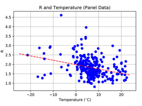
The paper concerned can be found here from which the key figure is this:
This plots the basic reproductive rateR against temperature for Coronavirus infections from 100 Chinese cities. The argument is that the trend means that higher temperatures correspond to weakened transmission of the virus (as happens with influenza). I don’t know if this paper has been peer-reviewed. I sincerely hope not!
I showed this plot to a colleague of mine the other day who remarked “well, at least all the points lie on a plane”. It looks to me that if if you removed just one point – the one with R>4.5 – then the trend would vanish completely.
The alleged correlation is deeply unimpressive on its own, quite apart from the assumption that any correlation present represents a causative effect due to temperature – there could be many confounding factors.
P.S. Among the many hilarious responses on Twitter was this:
Fitting a 36 degree polynomial rather than a straight line, it seems indeed that contagiousness decreases somewhat with temperature, but only until 23.5 ºC, after which it explodes!
In other words, your data show that we must take immediate action to avoid global warming! pic.twitter.com/57gBNavREe
Following the campaign for the forthcoming General Election in Ireland has confirmed (not entirely unexpectedly) that politicians over here are not averse to peddling demonstrable untruths.
One particular example came up in recent televised debate during which Fine Gael leader Leo Varadkar talked about his party’s plans for tax cuts achieved by raising the salary at which workers start paying the higher rate of income tax. Here’s a summary of the proposal from the Irish Times:
Fine Gael wants to increase the threshold at which people hit the higher rate of income tax from €35,300 to €50,000, which it says will be worth €3,000 to the average earner if the policy is fully implemented.
Three thousand (per year) to the average earner! Sounds great!
But let’s look at the figures. There are two tax rates in Ireland. The first part of your income up to a certain amount is taxed at 20% – this is known as the Standard Rate. The remainder of your income is taxed at 40% which is known as the Higher Rate. The cut-off point for the standard rate depends on circumstances, but for a single person it is currently €35,300.
According to official statistics the average salary is €38,893 per year, as has been widely reported. Let’s call that €38,900 for round figures. Note that figure includes overtime and other earnings, not just basic wages.
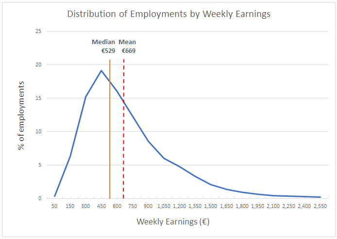
It’s worth pointing out that in Ireland (as practically everywhere else) the distribution of earnings is very skewed. here is an example showing weekly earnings in Ireland a few years ago to demonstrate the point.
This means that there are more people earning less than the average salary (also known as the mean) than above it. In Ireland over 60% of people earn less than the average. Using the mean in examples like this* is rather misleading – the median would be less influenced by a few very high salaries – but let’s continue with it for the sake of argument.
So how much will a person earning €38,900 actually benefit from raising the higher rate tax threshold to €50,000? For clarity I’ll consider this question in isolation from other proposed changes.
Currently such a person pays tax at 40% on the portion of their salary exceeding the threshold which is €38,900 – €35,300 = €3600. Forty per cent of that figure is €1440. If the higher rate threshold is raised above their earnings level this €3600 would instead be taxed at the Standard rate of 20%, which means that €720 would be paid instead of €1440. The net saving is therefore €720 per annum. This is a saving, but it’s nowhere near €3000. Fine Gael’s claim is therefore demonstrably false.
If you look at the way the tax bands work it is clear that a person earning over €50,000 would save an amount which is equivalent to 20% of the difference between €35,300 and €50,000 which is a sum close to €3000, but that only applies to people earning well over the average salary. For anyone earning less than €50,000 the saving is much less.
The untruth lies therefore in the misleading use of the term `average salary’.
Notice furthermore that anyone earning less than the higher rate tax threshold will not benefit in any way from the proposed change, so it favours the better off. That’s not unexpected for Fine Gael. A fairer change (in my view) would involve increasing the higher rate threshold and also the higher rate itself.
All this presupposes of course that you think cutting tax is a good idea at this time. Personally I don’t. Ireland is crying out for greater investment in public services and infrastructure so I think it’s inadvisable to make less money available for these purposes, which is what cutting tax would do.
*Another example is provided by the citation numbers for papers in the Open Journal of Astrophysics. The average number of citations for the 12 papers published in 2019 was around 34 but eleven of the twelve had fewer citations than this: the average is dragged up by one paper with >300 citations.
I have to admit I haven’t really kept up with developments in the world of gravitational waves this summer, though there have been a number of candidate events reported in the third observing run (O3) of Advanced LIGO which began in April 2019 to which I refer you if you’re interested.
The LIGO Scientific Collaboration and the Virgo Collaboration have cataloged eleven confidently detected gravitational-wave events during the first two observing runs of the advanced detector era. All eleven events were consistent with being from well-modeled mergers between compact stellar-mass objects: black holes or neutron stars. The data around the time of each of these events have been made publicly available through the Gravitational-Wave Open Science Center. The entirety of the gravitational-wave strain data from the first and second observing runs have also now been made publicly available. There is considerable interest among the broad scientific community in understanding the data and methods used in the analyses. In this paper, we provide an overview of the detector noise properties and the data analysis techniques used to detect gravitational-wave signals and infer the source properties. We describe some of the checks that are performed to validate the analyses and results from the observations of gravitational-wave events. We also address concerns that have been raised about various properties of LIGO-Virgo detector noise and the correctness of our analyses as applied to the resulting data.
It’s an interesting paper that gives quite a lot of detail, especially about signal extraction and parameter-fitting, so it’s very well worth reading.
Two particular things caught my eye about this. One is that there’s no list of authors anywhere in the paper, which seems a little strange. This policy may not be new, of course. I did say I haven’t really been keeping up.
The other point I’ll mention relates to this Figure, the caption of which refers to paper [41], the famous `Danish paper‘:
The Fourier phase is plotted vertically (between 0 and 2π) and the frequency horizontally. A random-phase distribution should have the phases uniformly distributed at each frequency. I think we can agree, without further statistical analysis, that the blue points don’t have that property! Of course nobody denies that the strongly correlated phases in the un-windowed data are at least partly an artifact of the application of a Fourier transform to a non-stationary time series.
I suppose by showing that using a window function to apodize the data removes phase correlations is meant to represent some form of rebuttal of the claims made in the Danish paper. If so, it’s not very convincing.
For a start the caption just says that after windowing resulting `phases appear randomly distributed‘. Could they not provide some more meaningful statistical statement than a simple eyeball impression? The text says little more:
In addition to causing spectral leakage, improper windowing of the data can result in spurious phase correlations in the Fourier transform. Figure 4 shows a scatter plot of the Fourier phase as a function of frequency … both with and without the application of a window function. The un-windowed data shows a strong phase correlation, while the windowed data does not.
(I added the link to the explanation of `spectral leakage’.)
As I have mentioned before on this blog, the human eye is very poor at distinguishing pattern from randomness. There are some subtleties involved in testing for correlated phases (e.g. because they are periodic) but there are various techniques available: I’ve worked on this myself (see, e.g., here and here.). The phases shown may well be consistent with a uniform random distribution, but I’m surprised the LIGO authors didn’t present a proper statistical analysis of the windowed phases to prove beyond doubt the point they seem to be trying to make.
Then again, later on in the caption, there is a statement that `the phases show some clustering around the 60 Hz power line’. So, on the one hand the phases `appear random’, but on the other hand they’re not. There are other plausible clusters elsewhere too. What about them?
I’m afraid the absence of quantitative detail means I don’t find this a very edifying discussion!
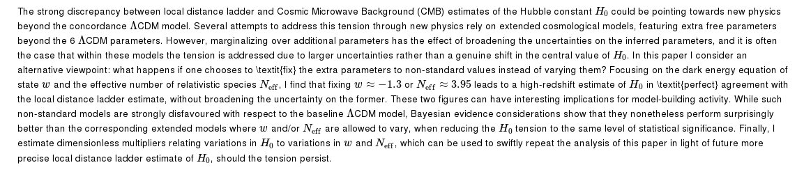
There was a new paper last week on the arXiv by Sunny Vagnozzi about the Hubble constant controversy (see this blog passim). I was going to refrain from commenting but I see that one of the bloggers I follow has posted about it so I guess a brief item would not be out of order.
Here is the abstract of the Vagnozzi paper:
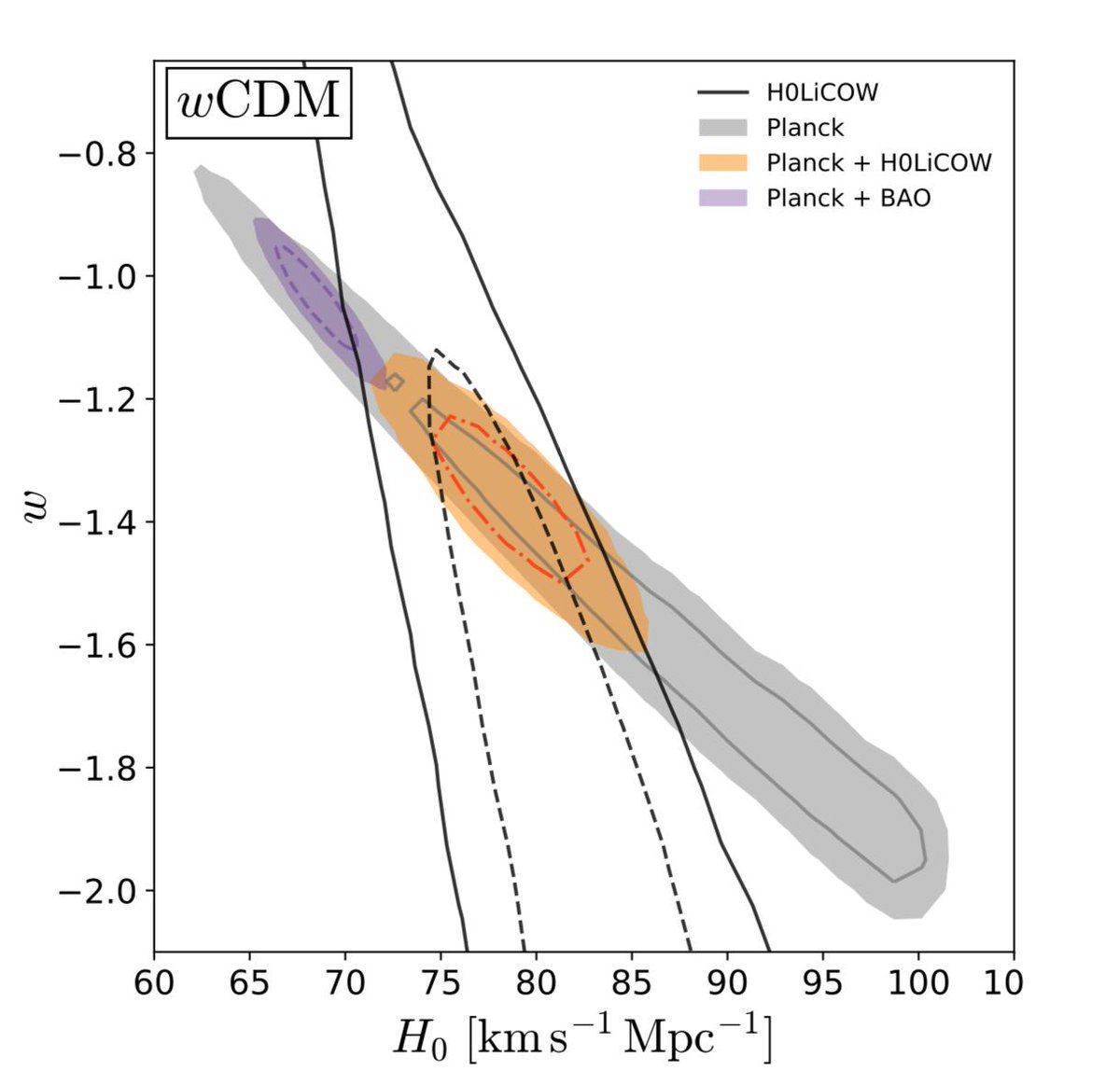
I posted this picture last week which is relevant to the discussion:
The point is that if you allow the equation of state parameter w to vary from the value of w=-1 that it has in the standard cosmology then you get a better fit. However, it is one of the features of Bayesian inference that if you introduce a new free parameter then you have to assign a prior probability over the space of values that parameter could hold. That prior penalty is carried through to the posterior probability. Unless the new model fits observational data significantly better than the old one, this prior penalty will lead to the new model being disfavoured. This is the Bayesian statement of Ockham’s Razor.
The Vagnozzi paper represents a statement of this in the context of the Hubble tension. If a new floating parameter w is introduced the data prefer a value less than -1 (as demonstrated in the figure) but on posterior probability grounds the resulting model is less probable than the standard cosmology for the reason stated above. Vagnozzi then argues that if a new fixed value of, say, w = -1.3 is introduced then the resulting model is not penalized by having to spread the prior probability out over a range of values but puts all its prior eggs in one basket labelled w = -1.3.
This is of course true. The problem is that the value of w = -1.3 does not derive from any ab initio principle of physics but by a posteriori of the inference described above. It’s no surprise that you can get a better answer if you know what outcome you want. I find that I am very good at forecasting the football results if I make my predictions after watching Final Score…
Indeed, many cosmologists think any value of w < -1 should be ruled out ab initio because they don’t make physical sense anyway.
The views presented here are personal and not necessarily those of my employer (or anyone else for that matter).
Feel free to comment on any of the posts on this blog but comments may be moderated; anonymous comments and any considered by me to be vexatious and/or abusive and/or defamatory will not be accepted. I do not necessarily endorse, support, sanction, encourage, verify or agree with the opinions or statements of any information or other content in the comments on this site and do not in any way guarantee their accuracy or reliability.