Exploitation

Posted in Poetry, Science Politics with tags , , on October 27, 2009 by telescoper

At the last Meeting of the RAS Council on October 9th 2009, Professor Keith Mason, Chief Executive of the Science and Technology Facilities Council (STFC), made a presentation after which he claimed that STFC spends too much on “exploitation”, i.e. on doing science with the facilities it provides. This statement clearly signals an intention to cut grants to research groups still further and funnel a greater proportion of STFC’s budget into technology development rather than pure research.

Following on from Phillip Helbig’s challenge a couple of posts ago, I decided to commemorate the occasion with an appropriate sonnet, inspired by Shakespeare’s Sonnet 14.

TO.THE.ONLIE.BEGETTER.OF.THIS.INSU(LT)ING.SONNET.

Mr K.O.M.

It seems Keith Mason doesn’t give a fuck
About the future of Astronomy.
“The mess we’re in is down to rotten luck
And our country’s  ruin’d economy”;
Or that’s the tale our clueless leader tells
When oft by angry critics he’s assailed,
Undaunted he in Swindon’s office dwells
Refusing to accept it’s him that failed.
And now he tells us we must realise:
We spend “too much on science exploitation”.
Forget the dreams of research in blue skies
The new name of the game is wealth creation.
A truth his recent statement underlines
Is that we’re doomed unless this man resigns.

Automatonophobia

Posted in Biographical with tags , , , on October 25, 2009 by telescoper

OK. I admit it. I’m  automatonophobic.

I don’t think I have many irrational fears. I don’t like snakes, and am certainly a bit frightened of them, but there’s nothing irrational about that. They’re nasty and likely to be poisonous. I don’t like slugs either, especially when they eat things in my garden. They’re unpleasant but easy to deal with and I’m not at all scared of them. Likewise spiders and insects.

But  ventriloquists’ dummies give me nightmares every time.

 When I was a little boy my grandfather took me to the Spanish City in Whitley Bay. There was an amusement arcade there and one of the attractions was thing called   The Laughing Sailor. You put a penny in the slot and a hideous  automaton  – very similar to the dummy a ventriloquist might use, except in mock-nautical attire – began to lurch backwards and forwards, flailing its arms, staring maniacally and emitting a loud mechanical cackle that was supposed to represent a laugh. The minute it started doing its turn I burst into tears and ran screaming out of the building. I’ve hated such things ever since.

The anxiety that these objects induce has now been given a name: automatonophobia, which is defined as “a persistent, abnormal, and unwarranted fear of ventriloquist’s dummies, animatronic creatures or wax statues”. Abnormal? No way. They’re simply horrible.

I’m clearly not the only one who thinks so, because there was an article in The Independent a few years ago by Neil Norman that exactly expressed the fear and loathing I feel about these creepy little dolls. Feature films  including Magic and Dead of Night, and episodes of The Twilight Zone and Hammer House of Horror have taken it further by playing with the idea that  a ventriloquist’s dummy has been possessed by some sort of malign power which  uses it to wreak terror on those around.

 We’re not talking about a benign wooden doll like Pinocchio who metamorphoses into a real boy; we’re talking about a ghastly staring-faced mannequin that is brought to life by its operator, the ventriloquist,  by inserting his hand up its backside. The dummy never looks human, but can speak and displays some human traits, usually nasty ones. The essence of a ventriloquist act is to generate the illusion  that one is watching two personalities sparring with each other when in reality the two voices are coming from the same person. Schizophrenia here we come.

It must be very clever to be able to throw your voice,  but I always had the nagging suspicion that ventriloquists use dummies to express the things they find it difficult to say through their own mouth, and so to give life to their darkest thoughts. 

Best of all the attempts to realise the sinister potential of this relationship in a movie is the “Ventriloquist’s Dummy” episode, directed by Alberto Cavalcanti, in Dead of Night, the 1945 portmanteau that some regard as Britain’s greatest horror film. Here is the part that tells  the tale of Michael Redgrave’s ventriloquist being sweatily possessed by the spirit of his malevolent dummy, Hugo. It’s old and creaky, but I find it absolutely terrifying.

So what is it about these man-child mannequins – they are always male – that makes them so creepy? First, there is their appearance: the mad, swivelling, psychotic eyes beneath arched eyebrows and that crude parody of a mouth (with painted teeth) that opens and shuts with a mechanical sound like a trap. Then there are the badly articulated limbs,  like those of a dead thing. When at rest,  their eyes remain open, their mouths fixed in a diabolic grimace. Moreover, with their rouged cheeks, lurid red lips and unnatural eyelashes, all ventriloquist’s dummies look like the badly embalmed corpses of small boys. And they always end up sitting on the knee of a horrible pervert.  Necrophilia and paedophilia all in one sick package. Yuck.

Worst of all, perhaps, is the voice. The high-pitched squawk that emerges is one of the most unpleasant sounds a human being can make. Even if you find it tolerable when you know that it comes from the ventriloquist, the last thing you want  is the dummy to start talking on its own.

I started writing this with the cathartic intention of exorcising the demon that appears whenever I see one of these wretched things. It didn’t work. However, I have now decided to take my mind off this track with a change of thread. Here’s a little quiz. I wonder if anyone can spot the connection between this post and the history of cosmology?

Alternatively, if you’re brave, you could try a bit of catharsis of your own and reveal your worst phobias through the comments box…

Stomp!

Posted in Jazz with tags , on October 24, 2009 by telescoper

I couldn’t resist a quick post about this old record, which was made in Chicago in 1928. The personnel line-up is very similar to that of the classic Hot Sevens, except that Louis Armstrong wasn’t there. Satchmo was, in fact, replaced for this number by two trumpeters, Natty Dominique and George Mitchell. John Thomas played trombone, Bud Scott was on banjo and Warren “Baby” Dodds played the drums.

The star of the show, however, is undoubtedly the great  Johnny Dodds (the older brother of the drummer). He was a clarinettist of exceptional power, a fact that enabled him to cut through the limitations of the relatively crude recording technology of the time. Standing shoulder-to-shoulder with Louis Armstrong doesn’t make it easy for a clarinettist to be heard!

This is still a favourite tune for jazz bands all around the world, but I’ve never heard a version as good as this one. There are lots of little things that contribute to its brilliance, such as the thumping 2/4 rhythm (which also gives away its origins in the New Orleans tradition of marching bands). It’s a bit fast to actually march to, though;  I suppose that’s what turns a march into a stomp. I like the little breaks too (such as Bud Scott’s banjo fill around 2:10 and, especially, the ensemble break at 2:45). But most of all it’s all about how they build up the momentum in such a  controlled way, using little key changes to shift gear but holding back until the time Johnny Dodds joins in again (around 2:20). At that point the whole thing totally catches fire and the remaining 40 seconds or so are some of the “hottest” in all of jazz history.

Some time ago I heard Robert Parker’s digitally remastered version of this track, which revealed that Baby Dodds was pounding away on the bass drum all the way through it. He’s barely audible on the original but it was clearly him that drove the performance along. Anyway, despite the relatively poor sound quality I do hope you enjoy it. It’s a little bit of musical history, but also an enormous bit of fun.

A Random Walk

Posted in The Universe and Stuff with tags , , , , , on October 24, 2009 by telescoper

In 1905 Albert Einstein had his “year of miracles” in which he published three papers that changed the course of physics. One of these is extremely famous: the paper that presented the special theory of relativity. The second was a paper on the photoelectric effect that led to the development of quantum theory. The third paper is not at all so well known. It was about the theory of Brownian motion.  In fact, Einstein spent an enormous amount of time and energy working on problems in statistical physics, something that isn’t so well appreciated these days as his work on the more glamorous topics of relativity and quantum theory.

 Brownian motion, named after the botanist Robert Brown,  is the perpetual jittering observed when small particles such as pollen grains are immersed in a fluid. It is now well known that these motions are caused by the constant bombardment of the grain by the fluid molecules. The molecules are too small to be seen directly, but their presence can be inferred from the visible effect on the much larger grain.

Brownian motion can be observed whenever  any relatively massive particles (perhaps large molecules) are immersed in a fluid comprising lighter particles. Here is a little video showing the Brownian motion observed by viewing smoke under a microscope. There is a small coherent “drift” motion in this example but superimposed on that you can clearly see the effect of gas atoms bombarding the (reddish) smoke particles:

The mathematical modelling of this process was pioneered by Einstein (and also Smoluchowski), but has now become a very sophisticated field of mathematics in its own right. I don’t want to go into too much detail about the modern approach for fear of getting far too technical, so I will concentrate on the original idea.

Einstein took the view that Brownian motion could be explained in terms of a type of stochastic process called a “random walk” (or sometimes “random flight”). I think the first person to construct a mathematical model to describethis type of phenomenon was the statistician Karl Pearson. The problem he posed concerned the famous drunkard’s walk. A man starts from the origin and takes a step of length L in a random direction. After this step he turns through a random angle and takes another step of length L. He repeats this process n times. What is the probability distribution for R, his total distance from the origin after these n steps? Pearson didn’t actually solve this problem, but posed it in a letter to Nature in 1905. Only a  week later, a reply from Lord Rayleigh was published in the same journal. He hadn’t worked it all out, written it up and sent it within a week though. It turns out that Rayleigh had solved essentially the same problem in a different context way back in 1880 so he had the answer readily available when he saw Pearson’s letter.

Pearson’s problem is a restricted case of a random walk, with each step having the same length. The more general case allows for a distribution of step lengths as well as random directions. To give a nice example for which virtually everything is known in a statistical sense, consider the case where each component of the step, i.e. x and y, are independent Gaussian variables, which have zero mean so that there is no preferred direction:

p(x)=\frac{1}{\sigma\sqrt{2\pi}} \exp \left(-\frac{x^2}{2\sigma^2}\right)  

A similar expression holds for p(y). Now we can think of the entire random walk as being two independent walks in x and y.  After n steps the total displacement in x, say, xn is given by

 p(x_n)=\frac{1}{\sigma\sqrt{n 2\pi }} \exp \left(-\frac{x_n^2}{2n\sigma^2}\right)

and again there is a similar expression for the distribution of yn . Notice that each of these distribution has a mean value of zero. On average, meaning on average over the entire probability distribution of realizations of the walk, the drunkard doesn’t go anywhere. In each individual walk he certainly does go somewhere, of course, but he is equally likely to move in any direction the probabilistic mean has to be zero. The total net displacement from the origin, rn , is just given by Pythagoras’ theorem:

r_n^2=x_n^2+y_n^2

 from which it is quite easy to establish that the probability distribution has to be

 p(r_n)=\frac{r_n}{n\sigma^2} \exp \left(-\frac{r_n^2}{2n\sigma^2}\right)

 This is called the Rayleigh distribution, and this kind of process is called a Rayleigh “flight”. The mean value of the displacement is just σ√n. By virtue of the ubiquitous central limit theorem, this result also holds in the original case discussed by Pearson in the limit of very large n. So this gives another example of the useful rule-of-thumb that quantities arising from fluctuations among n entities generally give a result that depends on the square root of n.

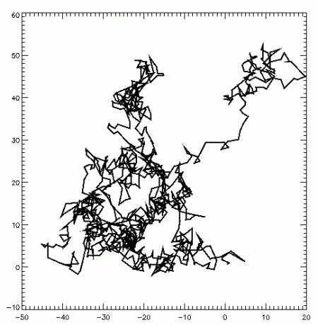
The figure below shows a simulation of a Rayleigh random walk. It is quite a good model for the jiggling motion executed by a Brownian particle. 

 sp003196

The step size resulting from a collision of a Brownian particle with a molecule depends on the mass of the molecule and of the particle itself. A heavier particle will be relatively unaffected by each bash and thus take longer to diffuse than a lighter particle. Here is a nice video showing three-dimensional simulations of the diffusion of sugar molecules (left) and proteins (right) that demonstrates this effect.

Of course not even the most inebriated boozer will execute a truly random walk. One would expect each step direction to have at least some memory of the previous one. This gives rise to the idea of a correlated random walk.  Such objects can be used to mimic the behaviour of geometric objects that possess some stiffness in their joints, such as proteins or other long molecules. Nowadays theory of Brownian motion and related stochastic phenomena is now considerably more sophisticated than the simply random flight models I have discussed here. The more general formalism can be used to understand many situations involving phenomena such as diffusion and percolation, not to mention gambling games and the stock market. The ability of these intrinsically “random” processes to yield surprisingly rich patterns is, to me, one of their most fascinating aspects. It takes only a little tweak to create order from chaos.


Nox Nocti Indicat Scientiam

Posted in Poetry, The Universe and Stuff with tags , on October 23, 2009 by telescoper

According to my blog access statistics, some of the poems I post on here seem to be fairly popular so I thought I’d put up another one by another poet  from the Metaphysical tradition, William Habington. He belonged to a prominent Catholic family and lived in England from 1605 to 1654, during a time of great religious upheaval.

The title of this particular poem is taken from the Latin (Vulgate) version of Psalm 19, the first two lines of which are

Caeli enarrant gloriam Dei et opus manus eius adnuntiat firmamentum.
Dies diei eructat verbum et nox nocti indicat scientiam.

The King James Bible translates this as

The heavens declare the glory of God; and the firmament sheweth his handywork.
Day unto day uttereth speech, and night unto night sheweth knowledge.

Some translations I have seen give “night after night” rather than the form above. My distant recollection of  Latin learnt at school tells me that nocti is the dative case of the third declension noun nox, so I think think “night shows knowledge to night” is indeed the correct sense of the Latin. Of course I don’t know what the sense of the original Hebrew is!

The original Psalm is the text on which one of the mightiest choruses of Haydn’s  Creation is based, “The Heavens are Telling” and Habington’s poem is a meditation on it. It seems to me to be a natural companion to the poem by John Masefield I posted earlier in the week, but I don’t know whether they share a common inspiration in the Psalm or just in the Universe itself.

When I survey the bright
Celestial sphere;
So rich with jewels hung, that Night
Doth like an Ethiop bride appear:

My soul her wings doth spread
And heavenward flies,
Th’ Almighty’s mysteries to read
In the large volumes of the skies.

For the bright firmament
Shoots forth no flame
So silent, but is eloquent
In speaking the Creator’s name.

No unregarded star
Contracts its light
Into so small a character,
Removed far from our human sight,

But if we steadfast look
We shall discern
In it, as in some holy book,
How man may heavenly knowledge learn.

It tells the conqueror
That far-stretch’d power,
Which his proud dangers traffic for,
Is but the triumph of an hour:

That from the farthest North,
Some nation may,
Yet undiscover’d, issue forth,
And o’er his new-got conquest sway:

Some nation yet shut in
With hills of ice
May be let out to scourge his sin,
Till they shall equal him in vice.

And then they likewise shall
Their ruin have;
For as yourselves your empires fall,
And every kingdom hath a grave.

Thus those celestial fires,
Though seeming mute,
The fallacy of our desires
And all the pride of life confute:–

For they have watch’d since first
The World had birth:
And found sin in itself accurst,
And nothing permanent on Earth.


Another take on cosmic anisotropy

Posted in Cosmic Anomalies, The Universe and Stuff with tags , , , on October 22, 2009 by telescoper

Yesterday we had a nice seminar here by Antony Lewis who is currently at Cambridge, but will be on his way to Sussex in the New Year to take up a lectureship there. I thought I’d put a brief post up here so I can add it to my collection of items concerning cosmic anomalies. I admit that I had missed the paper he talked about (by himself and Duncan Hanson) when it came out on the ArXiv last month, so I’m very glad his visit drew this to my attention.

What Hanson & Lewis did was to think of a number of simple models in which the pattern of fluctuations in the temperature of the cosmic microwave background radiation across the sky might have a preferred direction. They then construct optimal estimators for the parameters in these models (assuming the underlying fluctuations are Gaussian) and then apply these estimators to the data from the Wilkinson Microwave Anisotropy Probe (WMAP). Their subsequent analysis attempts to answer the question whether the data prefer these anisotropic models to the bog-standard cosmology which is statistically isotropic.

I strongly suggest you read their paper in detail because it contains a lot of interesting things, but I wanted to pick out one result for special mention. One of their models involves a primordial power spectrum that is intrinsically anisotropic. The model is of the form

P(\vec{ k})=P(k) [1+a(k)g(\vec{k})]

compared to the standard P(k), which does not depend on the direction of the wavevector. They find that the WMAP measurements strongly prefer this model to the standard one. Great! A departure from the standard cosmological model! New Physics! Re-write your textbooks!

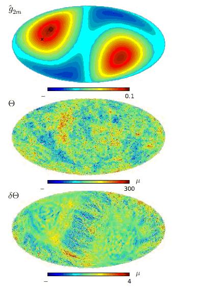
Well, not really. The direction revealed by the best-choice parameter fit to the data is shown in the smoothed picture  (top). Underneath it are simulations of the sky predicted by their  model decomposed into an isoptropic part (in the middle) and an anisotropic part (at the bottom).

lewis2

You can see immediately that the asymmetry axis is extremely close to the scan axis of the WMAP satellite, i.e. at right angles to the Ecliptic plane.

This immediately suggests that it might not be a primordial effect at all but either (a) a signal that is aligned with the Ecliptic plane (i.e. something emanating from the Solar System) or (b) something arising from the WMAP scanning strategy. Antony went on to give strong evidence that it wasn’t primordial and it wasn’t from the Solar System. The WMAP satellite has a number of independent differencing assemblies. Anything external to the satellite should produce the same signal in all of them, but the observed signal varies markedly from one to another. The conclusion, then, is that this particular anomaly is largely generated by an instrumental systematic.

The best candidate for such an effect is that it is an artefact of a asymmetry in the beams of the two telescopes on the satellite. Since the scan pattern has a preferred direction, the beam profile may introduce a direction-dependent signal into the data. No attempt has been made to correct for this effect in the published maps so far, and it seems to me to be very likely that this is the root of this particular anomaly.

We will have to see the extent to which beam systematics will limit the ability of Planck to shed further light on this issue.

I could not sleep for thinking of the sky

Posted in Poetry with tags , on October 21, 2009 by telescoper

A comment from another blogger about an item of mine containing another bit of poetry led me to put up this astronomy-inspired poem, by the former Poet Laureate John Masefield. It’s from a cycle called Lollingdown Downs, and is actually the 12th poem in the sequence. I hope you like it.

I could not sleep for thinking of the sky,
The unending sky, with all its million suns
Which turn their planets everlastingly
In nothing, where the fire-haired comet runs.

If I could sail that nothing, I should cross
Silence and emptiness with dark stars passing,
Then, in the darkness, see a point of gloss
Burn to a glow, and glare, and keep amassing,

And rage into a sun with wandering planets
And drop behind, and then, as I proceed,
See his last light upon his last moon’s granites
Die to a dark that would be night indeed.

Night where my soul might sail a million years
In nothing, not even death, not even tears.


It’s a PhD Jim, but not as we know it…

Posted in Uncategorized with tags , on October 19, 2009 by telescoper

A story in today’s WalesOnline, originally published in the Western Mail, inspired me to add a short item to this blog.

Mark Brake is a writer and broadcaster and Professor of Science Communication at the University of Glamorgan. According to the Western Mail, in May 2006 he completed a detailed tender for the Swindon-based RCPO – a professional procurement unit that works with seven of Britain’s research councils. Allegedly, in the 26-page document, Professor Brake  claimed to hold a doctorate with the title Astrophysics: Chemical Evolution of the Galaxies, awarded by University College Cardiff, the name held by Cardiff University until 1988. He never wrote such a thesis and holds no such degree.

The article goes on to say that the application was successful, and the University of Glamorgan was awarded £285,264 for a six-month Researchers in Residence project. Surprisingly, although the University of Glamorgan has not disputed the facts in the article, it has failed to return the money.

You will find no mention of this episode on Professor Brake’s  Wikipedia page, the content of which appears nevertheless to be hotly disputed.

Professor Brake, a self-styled “astrobiologist”, declined to comment on the article, but a comment on the WalesOnline site says it all:

It’s a PhD Jim……..but not as we know it………..

POSTSCRIPT 20th October 2009

The WalesOnline story has now been amended to state that the application was not successful. I am therefore happy to retract my criticism of the University of Glamorgan for failing to return the money, and accept that they never received it.

The rest of the story remains in place.

Moreover, here is the relevant part of page 19 of the 26-page document that was submitted to the RCPO. Apologies for the slightly wonky result of the scanning. It’s not ambiguous, and I have no reason to believe that it is a forgery.  Had Mark Brake been awarded a PhD then a copy of the thesis would be in the Cardiff University library (which it isn’t) and the National Library of Wales (which it isn’t). Either this document is a forgery or Professor Brake did indeed falsely represent his qualifications in the application.brake

Ergodic Means…

Posted in The Universe and Stuff with tags , , , , , , on October 19, 2009 by telescoper

The topic of this post is something I’ve been wondering about for quite a while. This afternoon I had half an hour spare after a quick lunch so I thought I’d look it up and see what I could find.

The word ergodic is one you will come across very frequently in the literature of statistical physics, and in cosmology it also appears in discussions of the analysis of the large-scale structure of the Universe. I’ve long been puzzled as to where it comes from and what it actually means. Turning to the excellent Oxford English Dictionary Online, I found the answer to the first of these questions. Well, sort of. Under etymology we have

ad. G. ergoden (L. Boltzmann 1887, in Jrnl. f. d. reine und angewandte Math. C. 208), f. Gr.

I say “sort of” because it does attribute the origin of the word to Ludwig Boltzmann, but the greek roots (εργον and οδοσ) appear to suggest it means “workway” or something like that. I don’t think I follow an ergodic path on my way to work so it remains a little mysterious.

The actual definitions of ergodic given by the OED are

Of a trajectory in a confined portion of space: having the property that in the limit all points of the space will be included in the trajectory with equal frequency. Of a stochastic process: having the property that the probability of any state can be estimated from a single sufficiently extensive realization, independently of initial conditions; statistically stationary.

As I had expected, it has two  meanings which are related, but which apply in different contexts. The first is to do with paths or orbits, although in physics this is usually taken to meantrajectories in phase space (including both positions and velocities) rather than just three-dimensional position space. However, I don’t think the OED has got it right in saying that the system visits all positions with equal frequency. I think an ergodic path is one that must visit all positions within a given volume of phase space rather than being confined to a lower-dimensional piece of that space. For example, the path of a planet under the inverse-square law of gravity around the Sun is confined to a one-dimensional ellipse. If the force law is modified by external perturbations then the path need not be as regular as this, in extreme cases wandering around in such a way that it never joins back on itself but eventually visits all accessible locations. As far as my understanding goes, however, it doesn’t have to visit them all with equal frequency. The ergodic property of orbits is  intimately associated with the presence of chaotic dynamical behaviour.

The other definition relates to stochastic processes, i.e processes involving some sort of random component. These could either consist of a discrete collection of random variables {X1…Xn} (which may or may not be correlated with each other) or a continuously fluctuating function of some parameter such as time t, i.e. X(t) or spatial position (or perhaps both).

Stochastic processes are quite complicated measure-valued mathematical entities because they are specified by probability distributions. What the ergodic hypothesis means in the second sense is that measurements extracted from a single realization of such a process have a definition relationship to analagous quantities defined by the probability distribution.

I always think of a stochastic process being like a kind of algorithm (whose workings we don’t know). Put it on a computer, press “go” and it spits out a sequence of numbers. The ergodic hypothesis means that by examining a sufficiently long run of the output we could learn something about the properties of the algorithm.

An alternative way of thinking about this for those of you of a frequentist disposition is that the probability average is taken over some sort of statistical ensemble of possible realizations produced by the algorithm, and this must match the appropriate long-term average taken over one realization.

This is actually quite a deep concept and it can apply (or not) in various degrees.  A simple example is to do with properties of the mean value. Given a single run of the program over some long time T we can compute the sample average

\bar{X}_T\equiv \frac{1}{T} \int_0^Tx(t) dt

the probability average is defined differently over the probability distribution, which we can call p(x)

\langle X \rangle \equiv \int x p(x) dx

If these two are equal for sufficiently long runs, i.e. as T goes to infinity, then the process is said to be ergodic in the mean. A process could, however, be ergodic in the mean but not ergodic with respect to some other property of the distribution, such as the variance. Strict ergodicity would require that the entire frequency distribution defined from a long run should match the probability distribution to some accuracy.

Now  we have a problem with the OED again. According to the defining quotation given above, ergodic can be taken to mean statistically stationary. Actually that’s not true. ..

In the one-parameter case, “statistically stationary” means that the probability distribution controlling the process is independent of time, i.e. that p(x,t)=p(x,t+Δt) . It’s fairly straightforward to see that the ergodic property requires that a process X(t) be stationary, but the converse is not the case. Not every stationary process is necessarily ergodic. Ned Wright gives an example here. For a higher-dimensional process, such as a spatially-fluctuating random field the analogous property is statistical homogeneity, rather than stationarity, but otherwise everything carries over.

Ergodic theorems are very tricky to prove in general, but there are well-known results that rigorously establish the ergodic properties of Gaussian processes (which is another reason why theorists like myself like them so much). However, it should be mentioned that even if the ergodic assumption applies its usefulness depends critically on the rate of convergence. In the time-dependent example I gave above, it’s no good if the averaging period required is much longer than the age of the Universe; in that case even ergodicity makes it difficult to make inferences from your sample. Likewise the ergodic hypothesis doesn’t help you analyse your galaxy redshift survey if the averaging scale needed is larger than the depth of the sample.

Moreover, it seems to me that many physicists resort to ergodicity when there isn’t any compelling mathematical grounds reason to think that it is true. In some versions of the multiverse scenario, it is hypothesized that the fundamental constants of nature describing our low-energy turn out “randomly” to take on different values in different domains owing to some sort of spontaneous symmetry breaking perhaps associated a phase transition generating  cosmic inflation. We happen to live in a patch within this structure where the constants are such as to make human life possible. There’s no need to assert that the laws of physics have been designed to make us possible if this is the case, as most of the multiverse doesn’t have the fine tuning that appears to be required to allow our existence.

As an application of the Weak Anthropic Principle, I have no objection to this argument. However, behind this idea lies the assertion that all possible vacuum configurations (and all related physical constants) do arise ergodically. I’ve never seen anything resembling a proof that this is the case. Moreover, there are many examples of physical phase transitions for which the ergodic hypothesis is known not to apply.  If there is a rigorous proof that this works out, I’d love to hear about it. In the meantime, I remain sceptical.

Au Privave

Posted in Jazz with tags , , , on October 18, 2009 by telescoper

At the risk of becoming a complete bore on the subject of bebop I thought I’d follow up an earlier post on the joys of jazz with this brilliant performance of yet another Charlie Parker tune, not by the man himself, but by one of his disciples.

I was lucky enough to hear Sonny Stitt live a number of times and he was always brilliant; he died in 1982. He was criticised by some jazz buffs between  numbers during one gig I was at with the words “You’re just playing like Charlie Parker!”, to which he replied by handing his alto saxophone to the twit  in the audience and saying “Here then. YOU play like Charlie Parker.”

Anyway, in the late 1950s (after Charlie Parker had died) Sonny Stitt sat in as on alto saxophone with the Oscar Peterson trio of which Ray Brown (bass) and Ed Thigpen (drums) were the other two members. They made a classic album for the Verve label which features a number of Charlie Parker numbers. Oscar Peterson isn’t my absolute favourite jazz pianist but it has to be said that he and his sidemen build up a colossal head of steam on these records, especially the one I’ve picked which is called Au Privave.

I tried for ages to unravel this intricate little tune. It’s basically a twelve-bar blues, but it is built  on much more complicated chords than the usual blues cycle. In its simplest form, the blues involves only three chords, the same three that most rock-and-roll tunes are built on. The foundation is a  “tonic” chord (T) based on the root note of whatever key it’s played in, often a basic triad consisting of the first, third and five notes of a major scale starting on that note or including the dominant 7th. The next chord is the subdominant chord  (S), shifting things up by a perfect fourth relative to the tonic, and then finally we have the dominant (D) which brings us up by a fifth from the original root note.

The basic twelve-bar blues has one chord per bar. The first four bars are accompanied by the tonic, then the subdominant S takes over for two bars followed by a return to the tonic for another two. The last four bars introduce the dominant (but only for one bar), followed by S for one and then back down to the root for the final two.

In a standard blues in F the sequence would thus be

| F| F| F |F | B♭| B♭| F| F | C| B♭| F| F|,

or possibly with F7 etc. The slow and relatively simple progression of chords gives these  blues a rather statuesque form: the soloist has to be really good to keep the thing going without getting bogged down. When played by a master even the simplest blues can be immensely powerful, but they can also be very dull when played not so well. It may be simple, but it certainly isn’t easy.

Au Privave is in F but has considerably more complicated changes than the bog-standard F blues. Parker inserted several intermediate chords to keep the harmonies moving and dispensed with some of the conventional progressions.  There are also more chords, usually two per bar rather than just one. The sequence here looks more like

| F| Gm7C7| F |Cm7F7| B♭| B♭| F7Gm7| Am7D7 | Gm7| C| FD7| G7C7|,

although I’m not sure I got them right as it tends to be played very fast! It’s a lot more to remember, but it’s also a much more dynamic setting  to improvise in which is what people like Charlie Parker wanted to create. Instead of moving quasi-statically through perfect intervals each chorus, you run helter-skelter through a constantly shifting harmonic environment. Notice also that there’s no comfortable return to the tonic at measure 12, even. The appearance of a C7 chord here is called a turnaround. Complicated? Yes, I suppose it is. But whenever I hear it played by Sonny Stitt it’s always just four minutes of sheer exhilaration.

Oh, and there’s another thing. Listen to the chorus that starts about 2:58. Did he really play all twelve bars without breathing?