When I give popular talks about Cosmology, I sometimes look for appropriate analogies or metaphors in television programmes about forensic science, such as CSI: Crime Scene Investigation which I watch quite regularly (to the disdain of many of my colleagues and friends). Cosmology is methodologically similar to forensic science because it is generally necessary in both these fields to proceed by observation and inference, rather than experiment and deduction: cosmologists have only one Universe; forensic scientists have only one scene of the crime. They can collect trace evidence, look for fingerprints, establish or falsify alibis, and so on. But they can’t do what a laboratory physicist or chemist would typically try to do: perform a series of similar experimental crimes under slightly different physical conditions. What we have to do in cosmology is the same as what detectives do when pursuing an investigation: make inferences and deductions within the framework of a hypothesis that we continually subject to empirical test. This process carries on until reasonable doubt is exhausted, if that ever happens.
Of course there is much more pressure on detectives to prove guilt than there is on cosmologists to establish the truth about our Cosmos. That’s just as well, because there is still a very great deal we do not know about how the Universe works.I have a feeling that I’ve stretched this analogy to breaking point but at least it provides some kind of excuse for writing about an interesting historical connection between astronomy and forensic science by way of the social sciences.

The gentleman shown in the picture on the left is Lambert Adolphe Jacques Quételet, a Belgian astronomer who lived from 1796 to 1874. His principal research interest was in the field of celestial mechanics. He was also an expert in statistics. In Quételet’s time it was by no means unusual for astronomers to well-versed in statistics, but he was exceptionally distinguished in that field. Indeed, Quételet has been called “the father of modern statistics”. and, amongst other things he was responsible for organizing the first ever international conference on statistics in Paris in 1853.
His fame as a statistician owed less to its applications to astronomy, however, than the fact that in 1835 he had written a very influential book which, in English, was titled A Treatise on Man but whose somewhat more verbose original French title included the phrase physique sociale (“social physics”). I don’t think modern social scientists would see much of a connection between what they do and what we do in the physical sciences. Indeed the philosopher Auguste Comte was annoyed that Quételet appropriated the phrase “social physics” because he did not approve of the quantitative statistical-based approach that it had come to represent. For that reason Comte ditched the term from his own work and invented the modern subject of sociology…
Quételet had been struck not only by the regular motions performed by the planets across the sky, but also by the existence of strong patterns in social phenomena, such as suicides and crime. If statistics was essential for understanding the former, should it not be deployed in the study of the latter? Quételet’s first book was an attempt to apply statistical methods to the development of man’s physical and intellectual faculties. His follow-up book Anthropometry, or the Measurement of Different Faculties in Man (1871) carried these ideas further, at the expense of a much clumsier title.
This foray into “social physics” was controversial at the time, for good reason. It also made Quételet extremely famous in his lifetime and his influence became widespread. For example, Francis Galton wrote about the deep impact Quételet had on a person who went on to become extremely famous:
Her statistics were more than a study, they were indeed her religion. For her Quételet was the hero as scientist, and the presentation copy of his “Social Physics” is annotated on every page. Florence Nightingale believed – and in all the actions of her life acted on that belief – that the administrator could only be successful if he were guided by statistical knowledge. The legislator – to say nothing of the politician – too often failed for want of this knowledge. Nay, she went further; she held that the universe – including human communities – was evolving in accordance with a divine plan; that it was man’s business to endeavour to understand this plan and guide his actions in sympathy with it. But to understand God’s thoughts, she held we must study statistics, for these are the measure of His purpose. Thus the study of statistics was for her a religious duty.
The person in question was of course Florence Nightingale. Not many people know that she was an adept statistician who was an early advocate of the use of pie charts to represent data graphically; she apparently found them useful when dealing with dim-witted army officers and dimmer-witted politicians.
The type of thinking described in the quote also spawned a number of highly unsavoury developments in pseudoscience, such as the eugenics movement (in which Galton himself was involved), and some of the vile activities related to it that were carried out in Nazi Germany. But an idea is not responsible for the people who believe in it, and Quételet’s work did lead to many good things, such as the beginnings of forensic science.
A young medical student by the name of Louis-Adolphe Bertillon was excited by the whole idea of “social physics”, to the extent that he found himself imprisoned for his dangerous ideas during the revolution of 1848, along with one of his Professors, Achile Guillard, who later invented the subject of demography, the study of racial groups and regional populations. When they were both released, Bertillon became a close confidante of Guillard and eventually married his daughter Zoé. Their second son, Adolphe Bertillon, turned out to be a prodigy.
Young Adolphe was so inspired by Quételet’s work, which had no doubt been introduced to him by his father, that he hit upon a novel way to solve crimes. He would create a database of measured physical characteristics of convicted criminals. He chose 11 basic measurements, including length and width of head, right ear, forearm, middle and ring fingers, left foot, height, length of trunk, and so on. On their own none of these individual characteristics could be probative, but it ought to be possible to use a large number of different measurements to establish identity with a very high probability. Indeed, after two years’ study, Bertillon reckoned that the chances of two individuals having all 11 measurements in common were about four million to one. He further improved the system by adding photographs, in portrait and from the side, and a note of any special marks, like scars or moles.
Bertillonage, as this system became known, was rather cumbersome but proved highly successful in a number of high-profile criminal cases in Paris. By 1892, Bertillon was exceedingly famous but nowadays the word bertillonage only appears in places like the Observer’s Azed crossword.
The main reason why Bertillon’s fame subsided and his system fell into disuse was the development of an alternative and much simpler method of criminal identification: fingerprints. The first systematic use of fingerprints on a large scale was implemented in India in 1858 in an attempt to stamp out electoral fraud.
The name of the British civil servant who had the idea of using fingerprinting in this way was Sir William James Herschel (1833-1917), the eldest child of Sir John Herschel, the astronomer, and thus the grandson of Sir William Herschel, the discoverer of Uranus. Another interesting connection between astronomy and forensic science.


 means the probability of A being true given the assumed truth of B; “AB” means “A and B”, etc. This basically follows from the fact that “A and B” must always be equivalent to “B and A”.


 . For a sample of size
  with
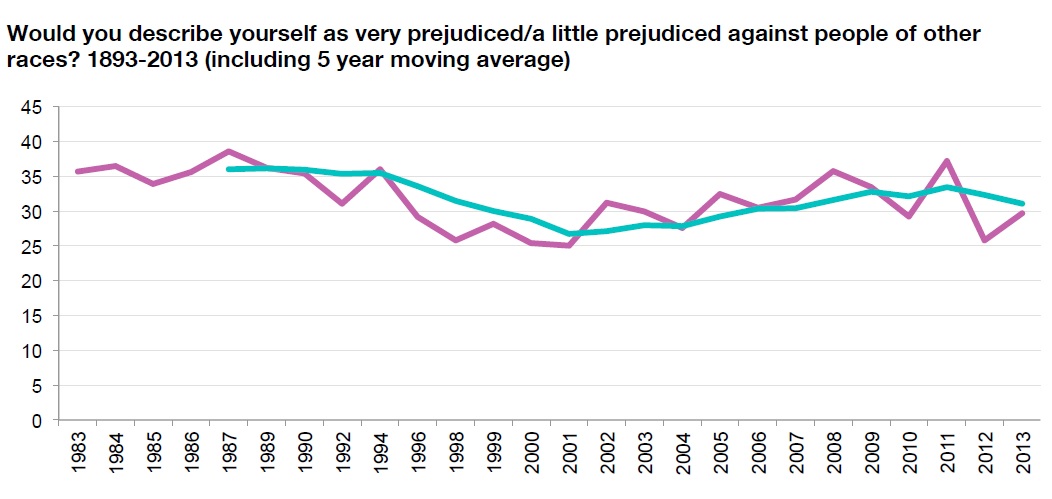
with  respondents indicating that they hen one can straightforwardly estimate
  . So far so good, as long as there is no bias induced by the form of the question asked nor in the selection of the sample, which for a telephone poll is doubtful.
 this amounts to a standard error of about 1.5%. About 95% of samples drawn from a population in which the true fraction is
  , i.e. within about 3% of the true figure. In other words the typical variation between two samples drawn from the same underlying population is about 3%.

 this amounts to a standard error of about 1%. About 95% of samples drawn from a population in which the true fraction is