It’s Saturday once again, so time for another update of activity at the Open Journal of Astrophysics. Since the last update we have published a further six papers, bringing the number in Volume 9 (2026) to 110 and the total so far published by OJAp up to 558.
I will continue to include the posts made on our Mastodon account (on Fediscience); these announcements also show the DOI for each paper.
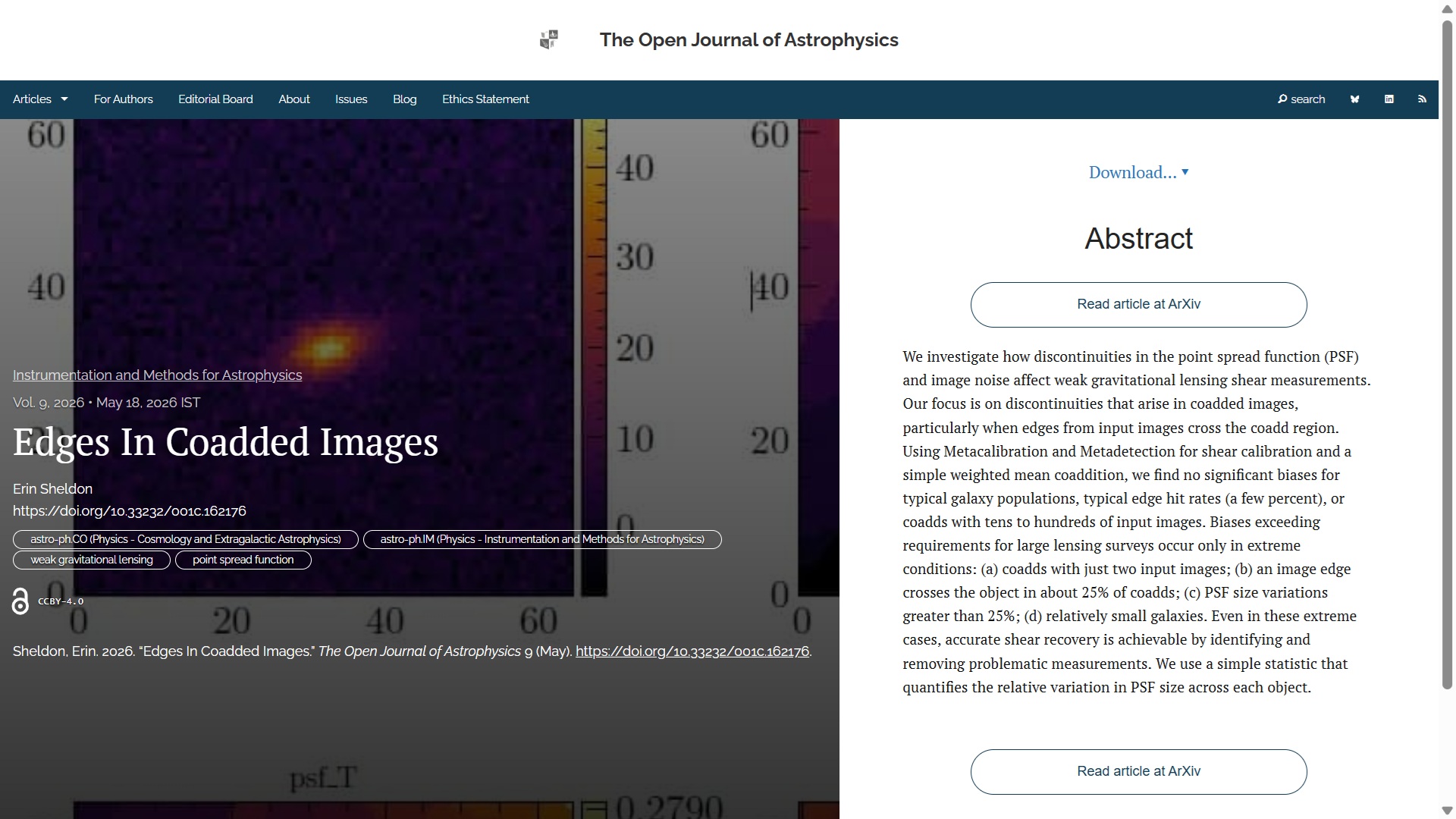
The first paper to report this week, published on Monday 18th May in the folder Instrumentation and Methods for Astrophysics is “Edges In Coadded Images” by Erin Sheldon (Brookhaven National Laboratory, USA). This paper describes a study exploring how image discontinuities and noise impact weak gravitational lensing measurements, finding no significant biases under typical conditions. Biases occur only in extreme cases, but can be mitigated.
The overlay for this paper is here
You can find the officially accepted version on arXiv here and the announcement on Fediverse here:

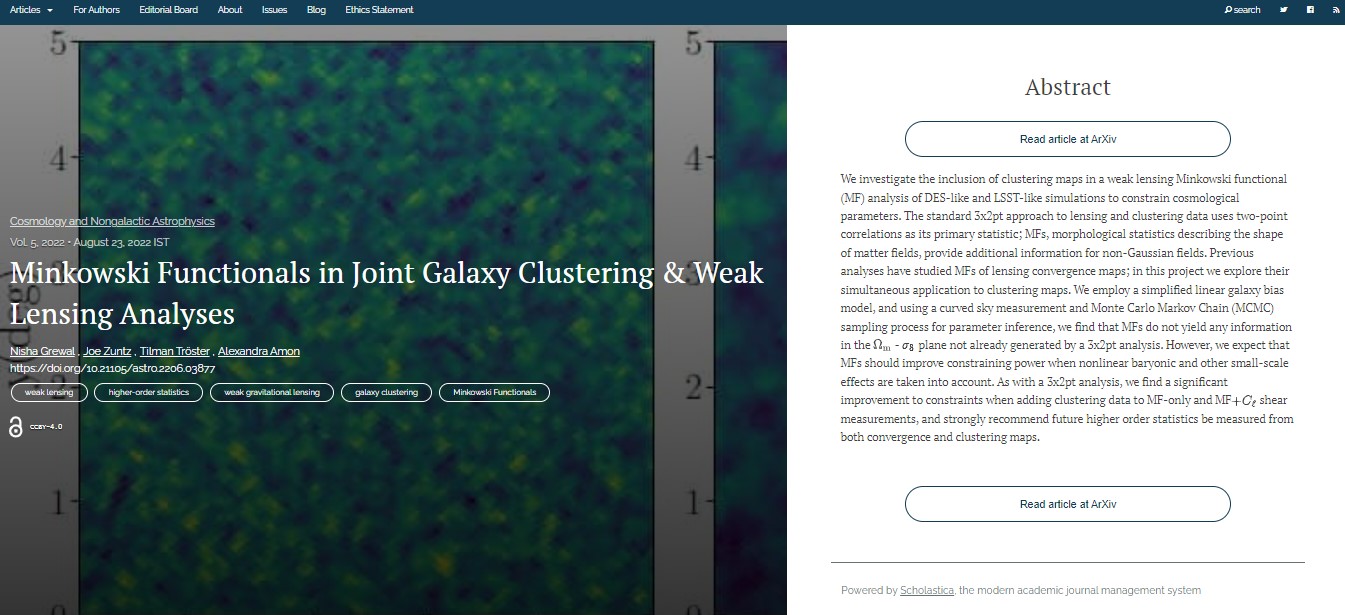
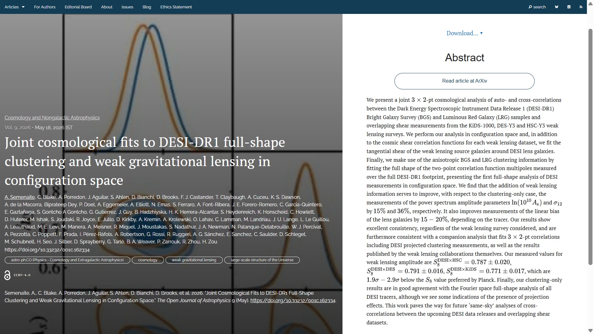
The second paper for this week, also published on Monday 18th May but in the folder Cosmology and Nongalactic Astrophysics, is “Joint cosmological fits to DESI-DR1 full-shape clustering and weak gravitational lensing in configuration space” by A. Semenaite (Swinburne Institute of Technology, Australia) and 72 other authors from all round the world. This paper presents a cosmological analysis of correlations between the DESI-DR1 Bright Galaxy Survey and Luminous Red Galaxy samples and overlapping shear measurements from various weak lensing surveys.
The overlay for this one is here:
The official version of the paper can be found on arXiv here and the Fediverse announcement here:
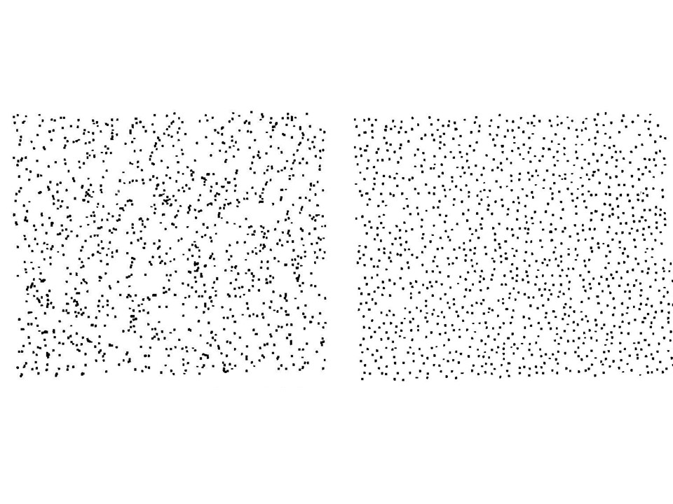
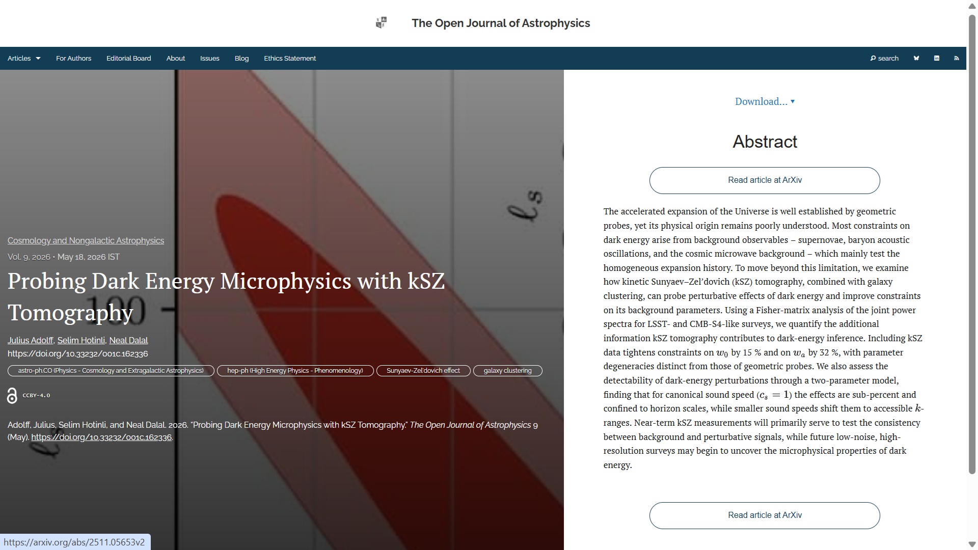
Next one up, the third paper of the week, and the third published on Monday 18th May, and in the folder Cosmology and Nongalactic Astrophysics is “Probing Dark Energy Microphysics with kSZ Tomography” by Julius Adolff, Selim Hotinli and Neal Dalal (all of the Perimeter Institute, Canada). This paper explores how kinetic Sunyaev-Zel’dovich tomography and galaxy clustering can enhance our understanding of dark energy and its effects, potentially revealing its microphysical properties in future surveys.
The overlay for this one is here:
The final, accepted version can be found on arXiv here and the Mastodon announcement is here:
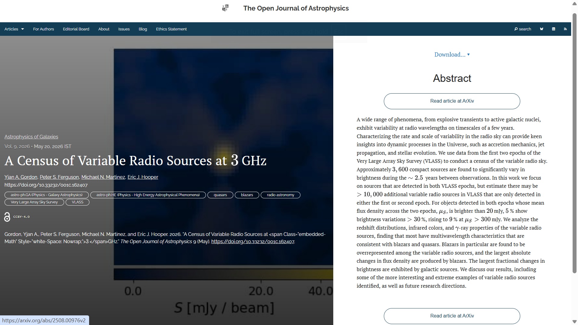
The fourth paper this week, published on Wednesday May 20th is “A Census of Variable Radio Sources at 3 GHz” by Yjan A. Gordon, Peter S. Ferguson, Michael N. Martinez and Eric J. Hooper (all of the University of Wisconsin, USA). This article, published in the folder Astrophysics of Galaxies, uses data from the Very Large Array Sky Survey to analyze variability in the radio sky, finding most changes consistent with blazars and quasars.
The overlay is here:
The officially accepted version can be found on arXiv here and here is the Mastodon announcement:
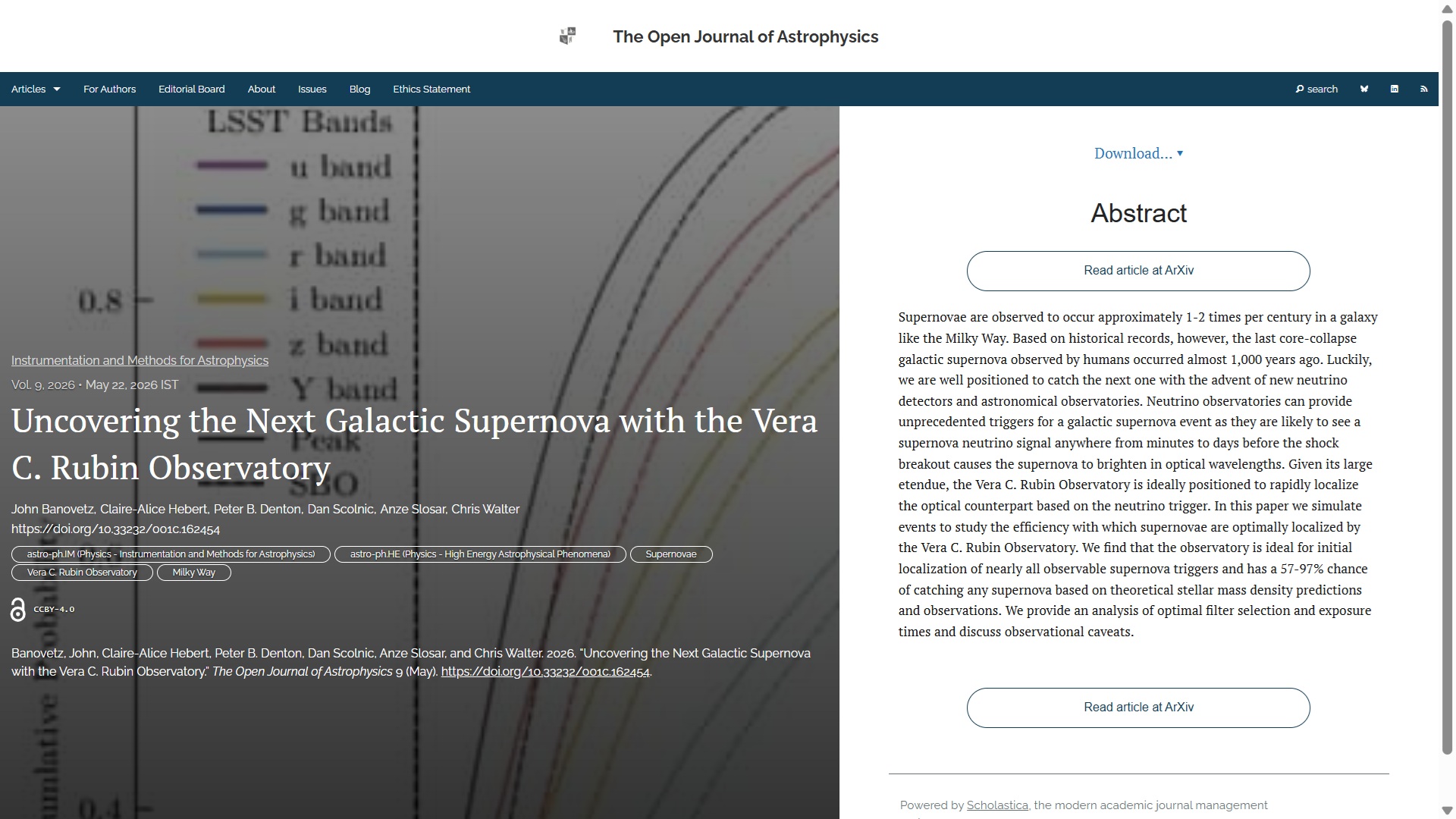
The fifth article of this week was published on Friday 22nd May in the folder Instrumentation and Methods for Astrophysics. The title is “Uncovering the Next Galactic Supernova with the Vera C. Rubin Observatory” by John Banovetz (Lawrence Berkeley Lab., USA), Claire-Alice Hebert & Peter B. Denton (Brookhaven National Lab., USA), Dan Scolnic (Duke University, USA), Anze Slosar (Brookhaven) and Chris Walter (Duke). The paper presents a study simulating how effectively the Vera C. Rubin Observatory can localize supernovae using neutrino triggers, finding a 57-97% success rate based on stellar mass density predictions.
The overlay is here:
You can find the authorized version of this paper on arXiv here and the Fediverse announcement is here:
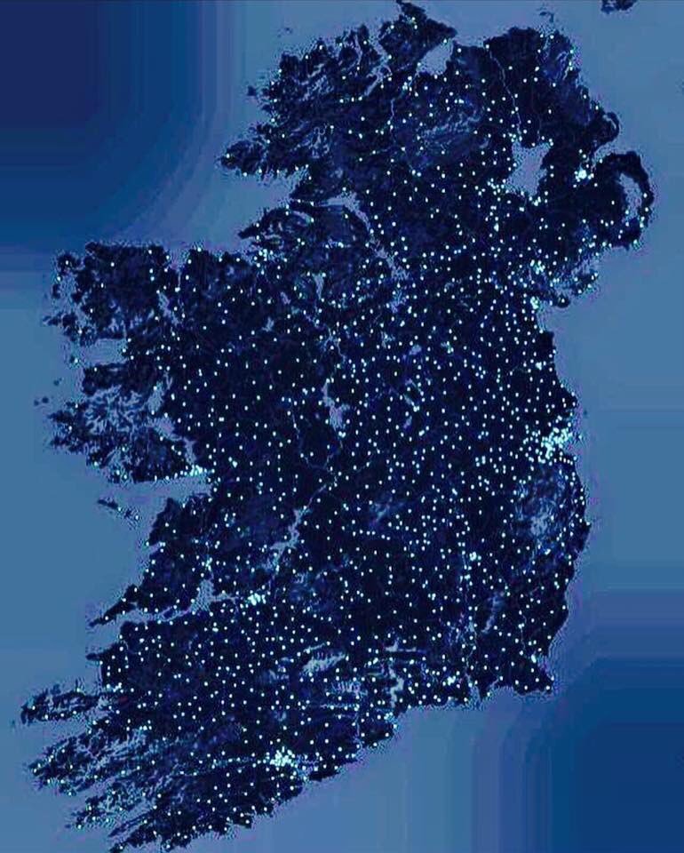
Last, but by no means least, this week we have “Pulsar timing solutions for 17 pulsars at 150 MHz from the Irish LOFAR station” by David J. McKenna (ASTRON, The Netherlands), Evan F. Keane (Trinity College Dublin, Ireland), Peter T. Gallagher (DIAS, Ireland) and Joe McCauley (Trinity). This was published on Friday 22nd May in the folder High-Energy Astrophysical Phenomena. It presents a demonstration of the use of international Low Frequency Array (LOFAR) stations in tracking and characterizing pulsars, providing new insights into these neutron stars’ emission properties.
The overlay for this one is here:
You can find the authorized version of this paper on arXiv here and the Fediverse announcement is here:
And that concludes this week’s update. I’ll do another one next Saturday.