Archive for WMAP

How Loud was the Big Bang?

Posted in The Universe and Stuff with tags , , , , , , on April 26, 2009 by telescoper

The other day I was giving a talk about cosmology at Cardiff University’s Open Day for prospective students. I was talking, as I usually do on such occasions, about the cosmic microwave background, what we have learnt from it so far and what we hope to find out from it from future experiments, assuming they’re not all cancelled.

Quite a few members of staff listened to the talk too and, afterwards, some of them expressed surprise at what I’d been saying, so I thought it would be fun to try to explain it on here in case anyone else finds it interesting.

As you probably know the Big Bang theory involves the assumption that the entire Universe – not only the matter and energy but also space-time itself – had its origins in a single event a finite time in the past and it has been expanding ever since. The earliest mathematical models of what we now call the  Big Bang were derived independently by Alexander Friedman and George Lemaître in the 1920s. The term “Big Bang” was later coined by Fred Hoyle as a derogatory description of an idea he couldn’t stomach, but the phrase caught on. Strictly speaking, though, the Big Bang was a misnomer.

Friedman and Lemaître had made mathematical models of universes that obeyed the Cosmological Principle, i.e. in which the matter was distributed in a completely uniform manner throughout space. Sound consists of oscillating fluctuations in the pressure and density of the medium through which it travels. These are longitudinal “acoustic” waves that involve successive compressions and rarefactions of matter, in other words departures from the purely homogeneous state required by the Cosmological Principle. The Friedman-Lemaitre models contained no sound waves so they did not really describe a Big Bang at all, let alone how loud it was.

However, as I have blogged about before, newer versions of the Big Bang theory do contain a mechanism for generating sound waves in the early Universe and, even more importantly, these waves have now been detected and their properties measured.

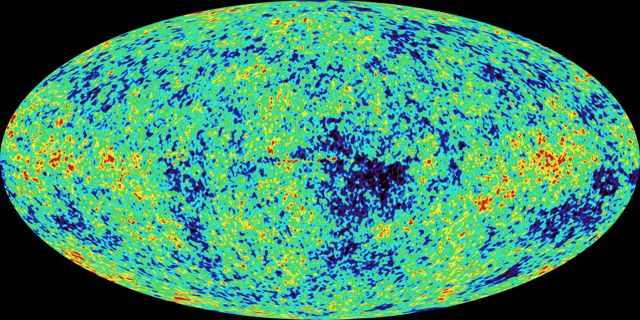
The above image shows the variations in temperature of the cosmic microwave background as charted by the Wilkinson Microwave Anisotropy Probe about five years ago. The average temperature of the sky is about 2.73 K but there are variations across the sky that have an rms value of about 0.08 milliKelvin. This corresponds to a fractional variation of a few parts in a hundred thousand relative to the mean temperature. It doesn’t sound like much, but this is evidence for the existence of primordial acoustic waves and therefore of a Big Bang with a genuine “Bang” to it.

A full description of what causes these temperature fluctuations would be very complicated but, roughly speaking, the variation in temperature you corresponds directly to variations in density and pressure arising from sound waves.

So how loud was it?

The waves we are dealing with have wavelengths up to about 200,000 light years and the human ear can only actually hear sound waves with wavelengths up to about 17 metres. In any case the Universe was far too hot and dense for there to have been anyone around listening to the cacophony at the time. In some sense, therefore, it wouldn’t have been loud at all because our ears can’t have heard anything.

Setting aside these rather pedantic objections – I’m never one to allow dull realism to get in the way of a good story- we can get a reasonable value for the loudness in terms of the familiar language of decibels. This defines the level of sound (L) logarithmically in terms of the rms pressure level of the sound wave Prms relative to some reference pressure level Pref

L=20 log10[Prms/Pref]

(the 20 appears because of the fact that the energy carried goes as the square of the amplitude of the wave; in terms of energy there would be a factor 10).

There is no absolute scale for loudness because this expression involves the specification of the reference pressure. We have to set this level by analogy with everyday experience. For sound waves in air this is taken to be about 20 microPascals, or about 2×10⁻¹⁰ times the ambient atmospheric air pressure which is about 100,000 Pa.  This reference is chosen because the limit of audibility for most people corresponds to pressure variations of this order and these consequently have L=0 dB. It seems reasonable to set the reference pressure of the early Universe to be about the same fraction of the ambient pressure then, i.e.

Pref~2×10⁻¹⁰ Pamb

The physics of how primordial variations in pressure translate into observed fluctuations in the CMB temperature is quite complicated, and the actual sound of the Big Bang contains a mixture of wavelengths with slightly different amplitudes so it all gets a bit messy if you want to do it exactly, but it’s quite easy to get a rough estimate. We simply take the rms pressure variation to be the same fraction of ambient pressure as the averaged temperature variation are compared to the average CMB temperature,  i.e.

Prms~ a few ×10-5Pamb

If we do this, scaling both pressures in logarithm in the equation in proportion to the ambient pressure, the ambient pressure cancels out in the ratio, which turns out to be a few times 10-5.

AudiogramsSpeechBanana

With our definition of the decibel level we find that waves corresponding to variations of one part in a hundred thousand of the reference level  give roughly L=100dB while part in ten thousand gives about L=120dB. The sound of the Big Bang therefore peaks at levels just over  110 dB. As you can see in the Figure above, this is close to the threshold of pain,  but it’s perhaps not as loud as you might have guessed in response to the initial question. Many rock concerts are actually louder than the Big Bang, at least near the speakers!

A useful yardstick is the amplitude  at which the fluctuations in pressure are comparable to the mean pressure. This would give a factor of about 1010 in the logarithm and is pretty much the limit that sound waves can propagate without distortion. These would have L≈190 dB. It is estimated that the 1883 Krakatoa eruption produced a sound level of about 180 dB at a range of 100 miles. By comparison the Big Bang was little more than a whimper.

PS. If you would like to read more about the actual sound of the Big Bang, have a look at John Cramer’s webpages. You can also download simulations of the actual sound. If you listen to them you will hear that it’s more of  a “Roar” than a “Bang” because the sound waves don’t actually originate at a single well-defined event but are excited incoherently all over the Universe.

Ecliptic Anomalies

Posted in Cosmic Anomalies, The Universe and Stuff with tags , , , , on February 12, 2009 by telescoper

Once a week the small band of cosmologists at Cardiff University have a little discussion group during which we look at an interesting and topical subject. Today my PhD student Rockhee chose an interesting paper by Diego et al entitled “WMAP anomalous signal in the ecliptic plane”. I thought I’d mention it here because it relates to an ongoing theme of mine, and I’ll refrain from commenting on the poor grammatical construction of the title.

The WMAP referred to is of course the Wilkinson Microwave Anisotropy Probe and I’ve blogged before about the tantalising evidence it suggests of some departures from the standard cosmological theory. These authors do something very simple and the result is extremely interesting.

In order to isolate the cosmic microwave background from foreground radiation produced in our own Galaxy, the WMAP satellite is equipped with receivers working at different frequencies. Galactic dust and free-free emission dominate the microwave sky temperature at high frequencies and Galactic synchotron takes over at low frequencies. The cosmic microwave background has the same temperature at all frequencies (i.e. it has a thermal spectrum) so it should be what’s left when the frequency-dependent bits are cleaned out.

What Diego et al. did was to make a map by combining the cleaned sky maps obtained at different frequencies obtained by WMAP in such a way as to try to eliminate the thermal (CMB) component. What is left when this is done should be just residual noise, as it should contain neither known foreground or CMB. The map they get is shown here.ecliptic

What is interesting is that the residual map doesn’t look like noise that is uniformly distributed over the sky: there are two distinct peaks close to the Ecliptic plane delineated by the black tramlines. Why the residuals look like this is a mystery. The peaks are both very far from the Galactic plane so it doesn’t look like they are produced by Galactic foregrounds.

One suggestion is that the anomalous signal is like an infra-red extension of the Zodiacal light (which is produced inside the Solar System and therefore is too local to be confined to the Galactic plane). The authors show, however, that a straightforward extrapolation of the known Zodiacal emission (primarily measured by the IRAS satellite) does not account for the signal seen in WMAP. If this is the explanation, then, there has to be a new source of Zodiacal emission that is not seen by IRAS but kicks in at WMAP frequencies.

Another possibility is that it is extragalactic. This is difficult to exclude, but is disfavoured in my mind because there is no a priori reason why it should be concentrated in the Ecliptic plane. Coincidences like this make me a bit uncomfortable. Some turn out to be real coincidences, but more often than not they are clues to something important. Agatha Christie would have agreed:

“Any coincidence,” said Miss Marple to herself, “is always worth noting. You can throw it away later if it is only a coincidence.”

On the other hand, the dipole asymmetry of the CMB (thought to be caused by our motion through a frame in which it is isotropic) is also lined up in roughly the same direction:

The dipole has a hot region and a cold region in places where the residual map has two hot regions and anyway it’s also a very large scale feature so the chances of it lining up by accident with the ecliptic plane to the accuracy seen is actually not small. Coincidences definitely do happen, and the rougher they are the more commonly they occur.

Obviously, I don’t know what’s going on, but  I will mention another explanation that might fit. As I have already blogged, the WMAP satellite scans the sky in a way that is oriented exactly at right angles to the Ecliptic plane. If there is an as yet unknown systematic error in the WMAP measurements, which is related in some way to the motion of the satellite, it could at least in principle produce an effect with a definite orientation with respect to the Ecliptic.

The only way we can rule out this (admittedly rather dull) explanation is by making a map using a different experiment. It’s good, then, that the Planck satellite is going to be launched in only a few weeks’ time (April 16th 2009). Fingers crossed that we can solve this riddle soon.

Power isn’t Everything

Posted in The Universe and Stuff with tags , , , , , , , on January 6, 2009 by telescoper

WMapThe picture above shows the latest available all-sky map of fluctuations in the temperature of the cosmic microwave background across the sky as revealed by the Wilkinson Microwave Anisotropy Probe, known to its friends as WMAP.

I’ve spent many long hours fiddling with the data coming from the WMAP experiment, partly because I’ve never quite got over the fact that such wonderful data actually exists. When I started my doctorate in 1985 the whole field of CMB analysis was so much pie in the sky, as no experiments had yet been performed with the sensitivity to reveal the structures we now see. This is because they are very faint and easily buried in noise. The fluctuations in temperature from pixel to pixel across the sky are of order one part in a hundred thousand of the mean temperature (i.e. about 30 microKelvin on a background temperature of about 3 Kelvin). That’s smoother than the surface of a billiard ball. That’s why it took such a long time to make the map shown above, and why it is such a triumphant piece of science.

I blogged a few days ago about the idea that the structure we see in this map was produced by sound waves reverberating around the early Universe. The techniques cosmologists use to analyse this sound are similar to those used in branches of acoustics except that we only see things in projection on the celestial sphere which requires a bit of special consideration.

One of the things that sticks in my brain from my undergraduate years is being told that if a physicist doesn’t know what they are doing they should start by making a Fourier transform. This breaks down the phenomenon being studied into a set of independent plane waves with different wavelengths corresponding to the different tones present in a complicated sound.

It’s often very good advice to do such a decomposition for one-dimensional time series or fluctuation fields in three-dimensional Cartesian space, even you do know what you’re doing, but it doesn’t work with a sphere because plane waves don’t fit properly on a curved surface. Fortunately, however, there is a tried-and-tested alternative involving spherical harmonics rather than plane waves.

Spherical harmonics are quite complicated beasts mathematically but they have pretty similar properties to Fourier harmonics in many respects. In particular they are represented as complex numbers having real and imaginary parts or, equivalently, an amplitude and a phase (usually called an argument by mathematicians). The latter representation is the most useful one for CMB fluctuations because the simplest versions of inflation predict that the phases of each of the spherical harmonic modes should be randomly distributed. What this really means is that there is no information content in their distribution so that the harmonic modes are in a state of maximum statistical disorder or entropy. This property also guarantees that the distribution of fluctuations over the sky should have a Gaussian distribution.

If you accept that the fluctuations are Gaussian then only the amplitudes of the spherical harmonic coefficients are useful. Indeed, their statistical properties can be specified entirely by the variance of these amplitudes as a function of mode frequency. This pre-eminently important function is called the power-spectrum of the fluctuations, and it is shown here for the WMAP data:

080999_powerspectrumm

Although the units on the axes are a bit strange it doesn”t require too much imagination to interpret this in terms of a sound spectrum. There is a characteristic tone (at the position of the peak) plus a couple of overtones. However these features are not sharp so the overall sound is not at all musical.

If the Gaussian assumption is correct then the power-spectrum contains all the useful statistical information to be gleaned from the CMB sky, which is why so much emphasis has been placed on extracting it accurately from the data.

Conversely, though, the power spectrum is completely insenstive to any information in the distribution of spherical harmonic phases. If something beyond the standard model made the Universe non-Gaussian it would affect the phases of the harmonic modes in a way that would make them non-random.

So far, so good. It sounds like it should be a straightforward job to work out whether the WMAP phases are random or not. Unfortunately, though, this task is heavily complicated by the presence of noise and systematics which can be quite easily cleaned from the spectrum but not from more sophisticated descriptors. All we can say so far is that the data seem to be consistent with a Gaussian distribution.

However, I thought I’d end with a bit of fun and show you how important phase information could actually be, if only we could find a good way of exploiting it. Let’s start with a map of the Earth, with the colour representing height of the surface above mean sea level:

sw_world

You can see the major mountain ranges (Andes, Himalayas) quite clearly as red in this picture and note how high Antarctica is…that’s one of the reasons so much astronomy is done there.

Now, using the same colour scale we have the WMAP data again (in Galactic coordinates).

sw_ilc

The virture of this map is that it shows how smooth the microwave sky is compared to the surface of the Earth. Note also that you can see a bit of crud in the plane of the Milky Way that serves as a reminder of the difficulty of cleaning the foregrounds out.

Clearly these two maps have completely different power spectra. The Earth is dominated by large features made from long-wavelength modes whereas the CMB sky has relatively more small-scale fuzz.

Now I’m going to play with these maps in the following rather peculiar way. First, I make a spherical harmonic transform of each of them. This gives me two sets of complex numbers, one for the Earth and one for WMAP. Following the usual fashion, I think of these as two sets of amplitudes and two sets of phases. Note that the spherical harmonic transformation preserves all the information in the sky maps, it’s just a different representation.

Now what I do is swap the amplitudes and phases for the two maps. First, I take the amplitudes of WMAP and put them with the phases for the Earth. That gives me the spherical harmonic representation of a new data set which I can reveal by doing an inverse spherical transform:

sw_worldphases

This map has exactly the same amplitudes for each mode as the WMAP data and therefore possesses an identical power spectrum to that shown above. Clearly, though, this particular CMB sky is not compatible with the standard cosmological model! Notice that all the strongly localised features such as coastlines appear by virtue of information contained in the phases but absent from the power-spectrum.

To understand this think how sharp features appear in a Fourier transform. A sharp spike at a specific location actually produces a broad spectrum of Fourier modes with different frequencies. These modes have to add in coherently at the location of the spike and cancel out everywhere else, so their phases are strongly correlated. A sea of white noise also has a flat power spectrum but has random phases. The key difference between these two configurations is not revealed by their spectra but by their phases.

Fortunately there is nothing quite as wacky as a picture of the Earth in the real data, but it makes the point that there are more things in Heaven and Earth than can be described in terms of the power spectrum!

Finally, perhaps in your mind’s eye you might consider what it might look lie to do the reverse experiment: recombine the phases of WMAP with the amplitudes of the Earth.

sw_ilcphases

If the WMAP data are actually Gaussian, then this map is a sort of random-phase realisation of the Earth’s power spectrum. Alternatively you can see that it is the result of running a kind of weird low-pass filter over the WMAP fluctuations. The only striking things it reveals are (i) a big blue hole associated with foreground contamination, (ii) a suspicious excess of red in the galactic plane owing to the same problem, and (iiI) a strong North-South asymmetry arising from the presence of Antarctica.

There’s no great scientific result here, just a proof that spherical harmonics can be fun.

PS. These pictures were made by a former PhD student of mine, Patrick Dineen, who has since quit astronomy to work in high finance. I hope he is weathering the global financial storm!