Archive for astronomy

Social Physics and Astronomy

Posted in The Universe and Stuff with tags , , , , , on March 23, 2009 by telescoper

When I give popular talks about Cosmology,  I sometimes look for appropriate analogies or metaphors in television programmes about forensic science, such as CSI: Crime Scene Investigation which I used to watch quite regularly (to the disdain of many of my colleagues and friends). Cosmology is methodologically similar to forensic science because it is generally necessary in both these fields to proceed by observation and inference, rather than experiment and deduction: cosmologists have only one Universe;  forensic scientists have only one scene of the crime. They can collect trace evidence, look for fingerprints, establish or falsify alibis, and so on. But they can’t do what a laboratory physicist or chemist would typically try to do: perform a series of similar experimental crimes under slightly different physical conditions. What we have to do in cosmology is the same as what detectives do when pursuing an investigation: make inferences and deductions within the framework of a hypothesis that we continually subject to empirical test. This process carries on until reasonable doubt is exhausted, if that ever happens.

Of course there is much more pressure on detectives to prove guilt than there is on cosmologists to establish the truth about our Cosmos. That’s just as well, because there is still a very great deal we do not know about how the Universe works.I have a feeling that I’ve stretched this analogy to breaking point but at least it provides some kind of excuse for writing about an interesting historical connection between astronomy and forensic science by way of the social sciences.

The gentleman shown in the picture on the left is Lambert Adolphe Jacques Quételet, a Belgian astronomer who lived from 1796 to 1874. His principal research interest was in the field of celestial mechanics. He was also an expert in statistics. In Quételet’s  time it was by no means unusual for astronomers to well-versed in statistics, but he  was exceptionally distinguished in that field. Indeed, Quételet has been called “the father of modern statistics”. and, amongst other things he was responsible for organizing the first ever international conference on statistics in Paris in 1853.


His fame as a statistician owed less to its applications to astronomy, however, than the fact that in 1835 he had written a very influential book which, in English, was titled A Treatise on Man but whose somewhat more verbose original French title included the phrase physique sociale (“social physics”).

Apparently the philosopher Auguste Comte was annoyed that Quételet appropriated the phrase “social physics” because he did not approve of the quantitative statistical-based  approach that it had come to represent. For that reason Comte  ditched the term from his own work and invented the subject of  sociology…

Quételet had been struck not only by the regular motions performed by the planets across the sky, but also by the existence of strong patterns in social phenomena, such as suicides and crime. If statistics was essential for understanding the former, should it not be deployed in the study of the latter? Quételet’s first book was an attempt to apply statistical methods to the development of man’s physical and intellectual faculties. His follow-up book Anthropometry, or the Measurement of Different Faculties in Man (1871) carried these ideas further, at the expense of a much clumsier title.

This foray into “social physics” was controversial at the time, for good reason. It also made Quételet extremely famous in his lifetime and his influence became widespread. For example, Francis Galton wrote about the deep impact Quételet had on a certain British lady:

Her statistics were more than a study, they were indeed her religion. For her Quételet was the hero as scientist, and the presentation copy of his “Social Physics” is annotated on every page. Florence Nightingale believed – and in all the actions of her life acted on that belief – that the administrator could only be successful if he were guided by statistical knowledge. The legislator – to say nothing of the politician – too often failed for want of this knowledge. Nay, she went further; she held that the universe – including human communities – was evolving in accordance with a divine plan; that it was man’s business to endeavour to understand this plan and guide his actions in sympathy with it. But to understand God’s thoughts, she held we must study statistics, for these are the measure of His purpose. Thus the study of statistics was for her a religious duty.

The name of the lady in question was Florence Nightingale. Not many people know that she was an adept statistician who was an early advocate of the use of pie charts to represent data graphically; she apparently found them useful when dealing with dim-witted army officers and dimmer-witted politicians.

The type of thinking described in the quote  also spawned a number of highly unsavoury developments in pseudoscience, such as the eugenics movement (in which Galton himself was involved), and some of the vile activities related to it that were carried out in Nazi Germany. But an idea is not responsible for the people who believe in it, and Quételet’s work did lead to many good things, such as the beginnings of forensic science.

A young medical student by the name of Louis-Adolphe Bertillon was excited by the whole idea of “social physics”, to the extent that he found himself imprisoned for his dangerous ideas during the revolution of 1848, along with one of his Professors, Achile Guillard, who later invented the subject of demography, the study of racial groups and regional populations. When they were both released, Bertillon became a close confidante of Guillard and eventually married his daughter Zoé. Their second son, Adolphe Bertillon, turned out to be a prodigy.

Young Adolphe was so inspired by Quételet’s work, which had no doubt been introduced to him by his father, that he hit upon a novel way to solve crimes. He would create a database of measured physical characteristics of convicted criminals. He chose 11 basic measurements, including length and width of head, right ear, forearm, middle and ring fingers, left foot, height, length of trunk, and so on. On their own none of these individual characteristics could be probative, but it ought to be possible to use a large number of different measurements to establish identity with a very high probability. Indeed, after two years’ study, Bertillon reckoned that the chances of two individuals having all 11 measurements in common were about four million to one. He further improved the system by adding photographs, in portrait and from the side, and a note of any special marks, like scars or moles.

Bertillonage, as this system became known, was rather cumbersome but proved highly successful in a number of high-profile criminal cases in Paris. By 1892, Bertillon was exceedingly famous but nowadays the word bertillonage only appears in places like the Observer’s Azed crossword.

The main reason why Bertillon’s fame subsided and his system fell into disuse was the development of an alternative and much simpler method of criminal identification: fingerprints. The first systematic use of fingerprints on a large scale was implemented in India in 1858 in an attempt to stamp out electoral fraud.

The name of the British civil servant who had the idea of using fingerprinting in this way was William Herschel, although I don’t think he was related to the astronomer of the same name.

That would be too much of a coincidence.

Factoid-based Learning

Posted in Books, Talks and Reviews, The Universe and Stuff with tags , on March 16, 2009 by telescoper

There’s a post over on cosmic variance that asks the question What is Scientific Literacy? Some of the comments reminded me of a book review I did for Nature a while ago, so I thought I’d put it on here.

My point is that teaching science isn’t about teaching facts, it’s about trying to develop critical thinking and problem-solving skills.
At least that’s what it should be, if only the dumbers-down would stop meddling.

BOOK REVIEWED Heavenly Errors: Misconceptions about the Real Nature of the Universe

by Neil F. Comins

Columbia University Press: 2001. 288 pp. $27.95, £18.95

Astronomy is a curious subject to teach. Even the most unpromising fledgling scientist has probably, at some stage, looked at the night sky and wondered about the meaning of it all. Students usually therefore enter the classroom with some preconceived notions about astronomical matters. These notions are often naïve, sometimes inaccurate, and occasionally downright bogus. The teaching of astronomy does not, therefore, begin with a blank piece of paper, as it does with other topics in physical science, but with the correction of misconceptions that may be deeply held.

In Heavenly Errors, Neil F. Comins illustrates the ambivalent consequences of astronomy’s peculiar allure with a series of commonly held misconceptions, misunderstandings and errors of logic. It is a promising idea for a book, particularly when the author has enlisted the willing help of thousands of undergraduate students to compile a list of frequently held wrong ideas about the Solar System and beyond. It is interesting to read of the origins of these misconceptions: Hollywood movies, astrology, the Internet and bad reporting of science all share some of the blame. But it’s even more interesting to look at the different kinds of misconception and what they tell us about the chasm that often lies between scientific thinking and the ‘common-sense’ reasoning they represent.

Ask why the weather is colder in the winter and you may well get the reply that, because its orbit is elliptical, the Earth is further from the Sun during winter than it is during summer and therefore receives less of the Sun’s power at that time of year. This explanation fails to explain why the Southern Hemisphere experiences summer at the same time as the Northern Hemisphere experiences winter, that is, at the same stage of the Earth’s orbit around the Sun. Talking through the logic of this example with students not only corrects the misconception, but also illustrates the scientific method by examining other necessary consequences of a given explanation before settling on the correct one. In this case, it is to do with the varying length of day and angle of the Sun in the sky.

Many of the examples presented by Comins are simple errors of fact. For example, “Polaris is the brightest star in the night sky”, comes in at number 8 in the top 50 Cosmic Clangers (it is Sirius). Many others do not justify being called misconceptions at all. Time travel, which Comins takes to be self-evidently impossible, is not, as he claims, excluded by the general theory of relativity. On the other hand, he states that black holes are definitely not black because they give off Hawking radiation — this despite the fact that Hawking radiation has not yet been observed in an astronomical object.

And what is a misconception anyway? Contrary to popular belief, planetary orbits are not circular, and yet circles provide a useful approximate description for many purposes. We are told that they are actually elliptical, but this is itself an approximation that ignores perturbations from other bodies and relativistic effects. Most scientific explanations are misconceptions if you view them like this.

Much of the early part of Heavenly Errors is excellent, particularly its explanations of the basic astronomical properties of the Sun, planets and comets. But further on, the book goes badly off the rails. Through its conflation of fact and theory, and its blurring of the distinction between truth and approximation, it turns into a misguided crusade that encourages the rote learning of factoids as a means to “acquire a sound scientific foundation for understanding nature”. I think this does more harm than good. T. H. Huxley, who knew a thing or two about science, put it best: “irrationally held truths may be more harmful than reasoned errors.”

The First Digit Phenomenon

Posted in Bad Statistics, The Universe and Stuff with tags , , on March 11, 2009 by telescoper

I thought it would be fun to put up this quirky example of how sometimes things that really ought to be random turn out not to be. It’s also an excuse to mention a strange connection between astronomy and statistics.

The astronomer Simon Newcomb (right) was born in 1835 in Nova Scotia picture2(Canada). He had no real formal education at all, but since there wasn’t much else to do in Nova Scotia, he taught himself mathematics and astronomy and became very adept at performing astronomical calculations with great diligence. He began work in a lowly position at the US Nautical Almanac Office in 1857, and by 1877 he was director. He became was professor of Mathematics and Astronomy and Johns Hopkins University from 1884 until 1893 and was made the first ever president of the American Astronomical Society in 1899; he died in 1909.
Newcomb was performing lengthy numerical calculations in an era long before the invention of the pocket calculator or desktop computer. In those days many such calculations, including virtually anything involving multiplication, had to be done using logarithms. The logarithm (to the base ten) of a number x is defined to be the number a such that x=10a. To multiply two numbers whose logarithms are a and b respectively involves simply adding the logarithms: 10a times 10b=10(a+b), which helps a lot because adding is a lot easier than multiplying if you have no calculator. The initial logarithms are simply looked up in a table; to find the answer you use different tables to find the “inverse” logarithm.

Newcomb was a heavy user of his book of mathematical tables for this type of calculation, and it became very grubby and worn. But he also noticed that the first pages of the logarithms seemed to have been used much more than the others. This puzzled him greatly. Logarithm tables are presented in order of the first digit of the number required: the first pages therefore contain logarithms for numbers beginning with the digit 1. Newcomb used the tables for a vast range of different calculations of different things. He expected the first digits of numbers that he had to look up to just be as likely to be anything. Shouldn’t they be randomly distributed? Shouldn’t all the pages be equally used?

Once raised, this puzzle faded away until it was re-discovered in 1938 and acquired the name of Benford’s law, or the first digit phenomenon. In virtually any list you can think of – street addresses, city populations, lengths of rivers, and so on – there are more entries beginning with the digit “1” than any other digit.

To give another example, although I admit this one is much harder to explain, in the American Physical Society’s list of fundamental constants, or at least the last version I happened to look at, no less than 40% begin with the digit 1. If you’ve been writing physics examination papers recently like I have, you will notice a similar behaviour. Out of the 16 physical constants listed in the rubric of a physics examination paper lying on my desk right now, 6 begin with the digit 1.

So what is going on?

There is a (relatively) simple answer, and a more complicated one. I’ll take the simple one first.

Consider street numbers in an address book as an example. Suppose Any street will be numbered from 1 to N. It doesn’t really matter what N is as long as it is finite (and nobody has ever built an infinitely long street). Now think about the first digits of the addresses. There are 9 possibilities, because we never start an address with 0. On the face of it, we might expect a fraction 1/9 (approximately 11%) of the addresses will start with 1. Suppose N is 200. What fraction actually starts with 1? The answer is more than 50%. Everything from 100 upwards, plus 1, and 11 to 19. Very few start with 9: only 9 itself, and 90-99 inclusive. If N is 300 then there are still more beginning with 1 than any other digit, and there are no more that start with 9. One only gets close to an equal fraction of each starting number if the value of N is an exact power of 10, e.g. 1000.

Now you can see why pulling numbers out of an address book leads to a distribution of first digits that is not at all uniform. As long as the numbers are being drawn from a collection of streets each of whom has a finite upper limit, then the result is bound to be biased towards low starting digits. Only if every street contained an exact power of ten addresses would the result be uniform. Every other possibility favours 1 at the start.

The more complicated version involves a scaling argument and is a more suitable explanation for the appearance of this phenomenon in measured physical quantities. Lengths, heights and weights of things are usually measured with respect to some reference quantity. In the absence of any other information, one might imagine that the distribution of whatever is being measured possesses some sort of invariance or symmetry with respect to the scale being chosen. In this case the prior distribution p(x) can be taken to have the so-called Jeffreys form, which is uniform in the logarithm, i.e. p(x) is proportional to 1/x. There obviously must be a cut-off at some point as this can’t be allowed to go on forever as it doesn’t converge for large x, but this doesn’t really matter for the sake of this argument. We can suppose anyway that there are many powers of ten involved before this upper limit is reached.

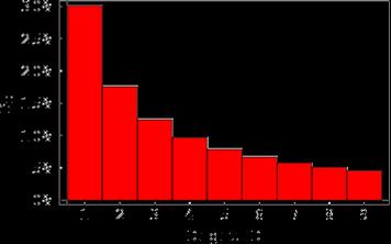
In this case the probability that the first digit is D is just given by the ratio of two terms: In the numerator we have the integral between D and D+1 of p(x) (that’s a measure of how much of the distribution represents numbers starting with the digit D) and on the denominator we have the integral between 1 and 10 of p(x) (the overall measure). The result, if we take p(x) to be proportional to 1/x, is just log (1+1/D).

picture1

The shape of this distribution is shown in the Figure. Note that about 30% of the first digits are expected to be 1. Of course I have made a number of simplifying assumptions that are unlikely to be exactly true, and the case of the physical constants is complicated by the fact that some are measured and some are defined, but I think this captures the essential reason for the curious behaviour of first digits.

If nothing else, it provides a valuable lesson that you should be careful in what variables you assume are uniformly distributed!

The Problem of the Steady State

Posted in Science Politics with tags , , on February 24, 2009 by telescoper

Just as a quick postscript to my recent item about proposed changes to the method of funding PhD students by STFC, let me point out the following simple calculation.

Assume that the number of permanent academic positions in a given field (e.g. astronomy) remains constant over time. If that is the case, each retirement (or other form of departure) from a permanent position will be replaced by one, presumably junior, scientist.

This means that over an academic career, on average, each academic will produce just one PhD who will get a permanent job. This of course doesn’t count students coming in from abroad, or those getting faculty positions abroad but in the case of the UK these are probably relatively small corrections.

Under the present supply of PhD studentships an academic can expect to get a PhD student at least once every three years or so. At a minimum, therefore, over a 30 year career one can expect to have ten PhD students. A great many supervisors have more PhD students than this, but this just makes the odds worse. The expectation is that only one of these will get a permanent job in the UK. The others (nine out of ten, according to my conservative estimate) above must either leave the field or the country to find permanent employment.

The arithmetic of this situation is a simple fact of life, but I’m not sure how many prospective PhD students are aware of it.

Scientiae Doctores

Posted in Science Politics with tags , , , on February 22, 2009 by telescoper

The season for recruiting new research students is well and truly upon us and at the same the Science & Technology Facilities Council (STFC) is consulting about changing the way that it allocates PhD studentships to departments.

Most postgraduate students studying for PhDs in Astronomy are funded by STFC (although some Universities also fund their own internal studentships). The result of this arrangement is that successful applicants to a PhD course can receive a stipend which amounts to about £13K per annum. It’s not a huge amount of money, but it is a stipend rather than a salary so it’s tax-free. Since a PhD student also remains a student and therefore qualifies for various other fringe benefits (Council Tax, student discounts, etc), it’s not actually a bad deal for the student. Anyway, if it were significantly more then it’s possible PhD students would have to start paying back their student loans, which would make things worse. STFC also pays a tuition fee to the University concerned, but this is done directly and the student doesn’t even see that element of the funding.

Since about 1995, PPARC and then STFC has funded research studentships in areas within its remit by means of peer review. Departments have bid for studentships (every two years) and a panel awards an allocation depending on the quality of the bid. Of course, everyone asks for many more studentships than are available so what you get is a fraction of what you ask for. I wrote the application for the first ever quota studentships for the Astronomy group at the University of Nottingham, and did it again a couple of times after that. Each time, despite going into best bullshit mode to write the case, I was frustrated by the relatively small number of studentships we were awarded. Although we succeeded in building up gradually from zero to 2-3 per year, it was a very slow process.

In recent years, the funding mechanism has evolved slightly so that studentship fees and stipends were devolved to the departments concerned in terms of Doctoral Training Grants (DTGs) rather than being administered centrally by PPARC/STFC. In the old days, students used to get their stipend from PPARC/STFC whereas now they are paid by their department from a cash grant.

Anyway, for various reasons (chief among them being no doubt to save administrative costs) STFC has decided to consult on changes to the mechanism for allocating the DTGs to the various departments around the country. The most serious proposed change is to follow the practice at the Engineering and Physical Sciences Research Council (EPSRC) and dispense with peer review. Instead, the proposal is to award studentships based on a formula involving how successful the department is at obtaining postdoctoral research assistant (PDRA) support from STFC.

Here is the proposed formula:

 Specifically, the studentship award per department should be proportional to the product of volume and average quality per academic within the department, that is to:


V * Q


The Committee has followed guidance in developing measures of V and Q that are non-subjective, repeatable and transparent.  The volume V is defined as the number of academics (including Fellows) eligible to hold STFC research grants. The  quality Q is measured by the number of STFC-funded PDRAs (P) awarded per academic (i.e. P/V), since this measures the success of the academic staff in securing STFC funding for PDRAs through peer-review.  More precisely we define quality per academic as Q = [1 +(P/V)].


Although the Committee felt this definition of quality applied primarily to responsive-mode PDRAs, it agreed that PDRAs on project grants should be included, but with a weighting, relative to responsive-mode, of 0.33.


Using these definitions, the Committee recommends that the studentship award per department should be proportional to a simple product of volume and average quality per academic within the department, that is to:


N(students) µ V * Q


where Q = [1 + (P/V)]


And so the departmental quota is proportional to: 


V[1+(P/V)] = V+P


In addition, recognising that very small departments offer more limited training opportunities on their own, a threshold is proposed, such that no studentships are awarded for V < 3. Instead, these very small departments/groups would be able to collaborate with other larger departments in seeking STFC studentship support.


Hence


         N(students) µ V+P  for V ³ 3

                             = 0        for V < 3


The constant of proportionality is chosen such that the total number of studentships equals the number available for allocation.


I think this is a fairly reasonable proposal, actually. The one thing I don’t really understand relates to the fact that STFC doesn’t just fund PDRAs on its grants, but under the Full Economic Cost regime (FEC), it also pays for fractions of academic staff effort for people working on its projects. On my recent successful STFC grant, for example, I was awarded 25% of my time (i.e. 0.25 FTE, full-time-equivalent) to do the research as well as a PDRA. Since the proposal above will have to cope with the question of what staff are “eligible” then why not make the quantity V proportional to the total FTEs funded, or at least only count those for whom some FEC time is allocated? And why not include staff FTE in the Q-factor too?

My guess is that such a modification wouldn’t make much difference to astronomy departments, but the original proposal has caused cries of anguish from particle physicists. This is because the number of PDRAs in particle physics is much smaller than in astronomy, so many large groups face a big reduction in their PhD quota. Including FEC numbers in the mix might well smooth the transition for them. For your information, the number of PDRAs per active astronomy researcher  is around 0.5 at present.

Anyway, the deadline for consulting on this has passed (on February 20th) so we now wait to see what STFC actually does. Probably the consultation period is a purely cosmetic exercise anyway and what will emerge is exactly what was proposed.

If you ask me (and nobody did), all this is mere tinkering. I think there are serious problems with graduate funding in the UK and these require much more radical remedies. At the risk of (and indeed with the intention of) being provocative, here is my diagnosis and suggested remedies:

  • There are too many PhDs in astronomy. STFC funded 160 studentships in 2006, compared with 88 in 2000. There are nowhere near enough PDRA positions to accommodate this number of PhDs in academic research. And even those who get their first PDRA position have very limited prospects of getting a permanent job. The result is a generation of disaffected students employed as low-paid assistants for 3-4 years and then thrown aside when they have got their PhD.
  • Of course, applicants for PhD places don’t know what research is really like and some will leave academia of their own volition when they find out that it’s not for them. In my experience, though, most graduate applicants simply don’t realise how heavily the odds are stacked against them. Less than one in ten can possibly stay in research in the long term, and the more PhDs are funded the worse the odds against them become.
  • The short duration of a British PhD disadvantages our students with respect to those from the USA or continental europe, who all do a lengthy Masters course before taking their PhD. These take at least 5 years to complete.  The result is that our home-grown PhDs are seriously disadvantaged in the job market against competitors from abroad. Similar points have been made forcefully by Ian Halliday.
  • My remedy is simple. Reduce the number of studentships but extend each one to five years and require each hosting department to provide a proper graduate school with intensive graduate-level courses to make up for the progressive reduction in content of undergraduate physics courses.
  • Even more unpopularly, I think the UK should scrap 4 years Masters (MPhys) programmes and embrace the structure of the Bologna agreement, i.e. a universal 3+2+3 structure of 3 years Bachelors, 2 years’ Masters and three years PhD.
  • Currently STFC stipends can only be paid to UK nationals and residents. It’s an open secret that most departments would preferentially recruit European physics graduates to their PhD positions if they were allowed to do so, because their undergraduate preparation is much better than that provided in UK universities. I propose that we abandon this protectionism and open up PhD opportunities to European applications, just as we would legally have to do if a PhD were considered to be a job.
  • Finally, I think the UK should consider the introduction of a common graduate entrance examination, perhaps based on the US GRE, to ensure the maintenance of appropriate standards for postgraduate entry and eligibility for STFC funding.

There are of course some advantages to the current British PhD system. For one thing, the PhD is earned very quickly. I was 25 when I got my PhD, and already had several publications. Most of my European collaborators were at least 30 before they got theirs (additional years have to be added for national service in many countries, but we don’t have it in the UK). But I am painfully aware that my technical knowledge outside the immediate area of my PhD is much thinner than most academics in the field. Now, in middle age, I feel like a long-distance runner who had inadequate preparation, went off too fast at the start of the race, and is now struggling along while people overtake him with monotonous regularity.

The nature of research in astronomy and cosmology has changed so much in the 20 years since I got my PhD that the old system has to go. Instead of tinkering with funding formula, driven principally by the need to save adminstrative costs within STFC, we need a radical overhaul of the entire graduate education system in the UK, involving all research councils and their political masters.

Unfortunately, though, for the time being at least the politicians have other more pressing matters to worry about, such the collapse of the economy.

What’s all the Noise?

Posted in Science Politics, The Universe and Stuff with tags , , , , on January 18, 2009 by telescoper

Now there’s a funny thing…

I’ve just come across a news item from last week which I followed up by looking at the official NASA press release. I’m very slow to pick up on things these days, but I thought I’d mention it anyway.

The experiment concerned is called ARCADE 2, which is an somewhat contrived acronym derived from Absolute Radiometer for Cosmology, Astrophysics and Diffuse Emission. It is essentially a balloon-borne detector designed to analyse radio waves with frequencies in the range 3 to 90 Ghz. The experiment actually flew in 2006, so it has clearly taken considerable time to analyse the resulting data.

Being on a balloon that flies for a relatively short time (2.5 hours in this case) means that only a part of the sky was mapped, amounting to about 7% of the whole celestial sphere but that is enough to map a sizeable piece of the Galaxy as well as a fairly representative chunk of deep space.

There are four science papers on the arXiv about this mission: one describes the instrument itself; another discusses radio emission from our own galaxy, the Milky Way; the third discusses the overall contribution of extragalactic origin in the frequency range covered by the instrument; the last discusses the implications about extragalactic sources of radio emission.

The thing that jumps out from this collection of very interesting science papers is that there is an unexplained, roughly isotropic, background of radio noise, consistent with a power-law spectrum. Of course to isolate this component requires removing known radio emission from our Galaxy and from identified extragalactic sources, as well as understanding the systematics of the radiometer during its flight. But after a careful analysis of these the authors present strong evidence of excess emission over and above known sources. The spectrum of this radio buzz falls quite steeply with frequency so appears in the two long-wavelength channels at 3 and 8 GHz.

So where does this come from? Well, we just don’t know.

The problem is that no sensible extrapolation of known radio sources to high redshift appears to be able to generate an integrated flux equivalent to that observed. Here is a bit of the discussion from the paper:

It is possible to imagine that an unknown population of discrete sources exist below the flux limit of existing surveys. We argue earlier that these cannot be a simple extension of the source counts of star-forming galaxies. As a toy model, we consider a population of sources distributed with a delta function in flux a factor of 10 fainter than the 8.4 GHz survey limit of Fomalont et al. (2002). At a flux of 0.75 μJy, it would take over 1100 such sources per square arcmin to produce the unexplained emission we see at 3.20 GHz, assuming a frequency index of −2.56. This source density is more than two orders of magnitude higher than expected from extrapolation to the same flux limit of the known source population. It is, however, only modestly greater than the surface density of objects revealed in the faintest optical surveys, e.g., the Hubble Ultra Deep Field (Beckwith et al. 2006).  The unexplained emission might result from an early population of non thermal emission from low-luminosity AGN; such a source would evade the constraint implied by the far-IR measurements.

The point is that ordinary galaxies produce a broad spectrum of radiation and it is difficult to boost the flux at one frequency without violating limits imposed at others. It might be able to invoke Active Galactic Nuclei (AGN) to do the trick, but I’m not sure. I am sure there’ll be a lot work going on trying to see how this might fit in with all the other things we know about galaxy formation and evolution but for the time being it’s a mystery.

I’m equally sure that these results will spawn a plethora of more esoteric theoretical explanations, inevitably including the ridiculous as well as perhaps the sublime. Charged dark matter springs to mind.

Or maybe it’s not even extragalactic. Could it be from an unknown source inside the Milky Way? If so, it might shed some light on the curiosities we find in the cosmic microwave background that I’ve mentioned here and there, but it seems to peak at too low a frequency to account for much of the overall microwave sky temperature.

But it does have a lesson for astronomy funders. ARCADE 2 is a very cheap experiment (by NASA standards). Moreover, the science goals of the experiment did not include “discovering a new cosmic background”. It just goes to show that even in these times of big, expensive and narrowly targetted missions there is still space for serendipity.

The Physics Overview

Posted in Science Politics with tags , , , , , , , , on January 17, 2009 by telescoper

I found out by accident the other day that the Panels conducting the 2008 Research Assessment Exercise have now published their subject overviews, in which they comment trends within each discipline.

Heading straight for the overview produced by the panel for Physics (which is available together with two other panels here),I found some interesting points, some of which relate to comments posted on my previous items about the RAE results (here and here) until I terminated the discussion.

One issue that concerns many physicists is how the research profiles produced by the RAE panel will translate into funding. I’ve taken the liberty of extracting a couple of paragraphs from the report to show what they think. (For those of you not up with the jargon, UoA19 is the Unit of Assessment 19, which is Physics).

The sub-panel is pleased with how much of the research fell into the 4* category and that this excellence is widely spread so that many smaller departments have their share of work assessed at the highest grade. Every submitted department to UoA19 had at least 70% of their overall quality profile at 2* or above, i.e. internationally recognised or above.

Sub-panel 19 takes the view that the research agenda of any group, or of any individual for that matter, is interspersed with fallow periods during which the next phase of the research is planned and during which outputs may be relatively incremental, even if of high scientific quality. In the normal course of events successful departments with a long term view will have a number of outputs at the 3* and 2* level indicating that the groundwork is being laid for the next set of 4* work. This is most obviously true for those teams involved with very major experiments in the big sciences, but also applies to some degree in small science. Thus the quality profile is a dynamic entity and even among groups of very high international standing there is likely to be cyclic variation in the relative amounts of 3* and 4* work according to the rhythm of their research programmes. Most departments have what we would consider a healthy balance between the perceived quality levels. The subpanel strongly believes that the entire overall profile should be considered when measuring the quality of a department, rather than focussing on the 4* component only.

I think this is very sensible, but for more reasons than are stated. For a start the judgement of what is 4* or 3* must be to some extent subjective and it would be crazy to allocate funding entirely according to the fraction of 4* work. I’ve heard informally that the error in any of the percentages for any assessment is plus or minus 10%, which also argues for a conservative formula. However one might argue about the outcome, the panels clearly spent a lot of time and effort determining the profiles so it would seem to make sense to use all the information they provide rather than just a part.

Curiously, though, the panel made no comment about why it is that physics came out so much worse than chemistry in the 2008 exercise (about one-third of the chemistry departments in the country had a profile-weighted quality mark higher than or equal to the highest-rated physics department). Perhaps they just think UK chemistry is a lot better than UK physics.

Anyway, as I said, the issue most of us are worrying about is how this will translate into cash. I suspect HEFCE hasn’t worked this out at all yet either. The panel clearly thinks that money shouldn’t just follow the 4* research, but the HEFCE managers might differ. If they do wish to follow a drastically selective policy they’ve got a very big problem: most physics departments are rated very close together in score. Any attempt to separate them using the entire profile would be hard to achieve and even harder to justify.

The panel also made a specific comment about Wales and Scotland, which is particularly interesting for me (being here in Cardiff):

Sub-panel 19 regards the Scottish Universities Physics Alliance collaboration between Scottish departments as a highly positive development enhancing the quality of research in Scotland. South of the border other collaborations have also been formed with similar objectives. On the other hand we note with concern the performance of three Welsh departments where strategic management did not seem to have been as effective as elsewhere.

I’m not sure whether the dig about Welsh physics departments is aimed at the Welsh funding agency HEFCW or the individual university groups; SUPA was set up with the strong involvement of SFC and various other physics groupings in England (such as the Midlands Physics Alliance) were actively encouraged by HEFCE. It is true, though, that the 3 active physics departments in Wales (Cardiff, Swansea and Aberystwyth) all did quite poorly in the RAE. In the last RAE, HEFCW did not apply as selective a funding formula as its English counterpart HEFCE with the result that Cardiff didn’t get as much research funding as it would if it had been in England. One might argue that this affected the performance this time around, but I’m not sure about this as it’s not clear how any extra funding coming into Cardiff would have been spent. I doubt if HEFCW will do any different this time either. Welsh politics has a strong North-South issue going on, so HEFCW will probably feel it has to maintain a department in the North. It therefore can’t penalise Aberystwyth too badly for its poor RAE showing. The other two departments are larger and had very similar profiles (Swansea better than Cardiff, in fact) so there’s very little justification for being too selective there either.

The panel remarked on the success of SUPA which received a substantial injection of cash from the Scottish Funding Council (SFC) and which has led to new appointments in strategic areas in several Scottish universities. I’m a little bit skeptical about the long-term benefits of this because the universities themselves will have to pick up the tab for these positions when the initial funding dries up. Although it will have bought them extra points on the RAE score the continuing financial viability of physics departments is far from guaranteed because nobody yet knows whether they will gain as much cash from the outcome as they spent to achieve it. The same goes for other universities, particularly Nottingham, who have massively increased their research activity with cash from various sources and consequently done very well in the RAE. But will they get back as much as they have put in? It remains to be seen.

What I would say about SUPA is that it has definitely given Scottish physics a higher profile, largely from the appointment of Ian Halliday to front it. He is an astute political strategist and respected scientist who performed impressively as Chief Executive of the now-defunct Particle Physics and Astronomy Research Council and is also President of the European Science Foundation. Having such a prominent figurehead gives the alliance more muscle than a group of departmental heads would ever hope to have.

So should there be a Welsh version of SUPA? Perhaps WUPA?

Well, Swansea and Cardiff certainly share some research interests in the area of condensed-matter physics but their largest activities (Astronomy in Cardiff, Particle Physics in Swansea) are pretty independent. It seems to me to be to be well worth thinking of some sort of initiative to pool resources and try to make Welsh physics a bit less parochial, but the question is how to do it. At coffee the other day, I suggested an initiative in the area of astroparticle physics could bring in genuinely high quality researchers as well as establishing synergy between Swansea and Cardiff, which are only an hour apart by train. The idea went down like a lead balloon, but I still think it’s a good one. Whether HEFCW has either the resources or the inclination to do something like it is another matter, even if the departments themselves were to come round.

Anyway, I’m sure there will be quite a lot more discussion about our post-RAE strategy if and when we learn more about the funding implications. I personally think we could do with a radical re-think of the way physics in Wales is organized and could do with a champion who has the clout of Scotland’s SUPA-man.

The mystery as far as I am concerned remains why Cardiff did so badly in the ratings. I think the first quote may offer part of the explanation because we have large groups in Astronomical Instrumentation and Gravitational Physics, both of which have very long lead periods. However, I am surprised and saddened by the fact that the fraction rated at 4* is so very low. We need to find out why. Urgently.

Professor Who?

Posted in Biographical, Music, Television, The Universe and Stuff with tags , , , , , on January 7, 2009 by telescoper

As a Professor of Astrophysics I am often asked “Why on Earth did you take up such a crazy subject?”

I guess many astronomers, physicists and other scientists have to answer this sort of question. For many of them there is probably a romantic reason, such as seeing the rings of Saturn or the majesty of the Milky Way on a dark night. Others will probably have been inspired by TV documentary series such as The Sky at Night, Carl Sagan’s Cosmos or even Horizon which, believe it or not, actually used to be quite good but which is nowadays uniformly dire. Or it could have been something a bit more mundane but no less stimulating such as a very good science teacher at school.

When I’m asked this question I’d love to be able to put my hand on my heart and give an answer of that sort but the truth is really quite a long way from those possibilities. The thing that probably did more than anything else to get me interested in science was a Science Fiction TV series or rather not exactly the series but the opening titles.

The first episode of Doctor Who was broadcast in the year of my birth, so I don’t remember it at all, but I do remember the astonishing effect the credits had on my imagination when I saw later episodes as a small child. Here are some tests for the sequence as it appeared in the very first series featuring William Hartnell as the first Doctor.

To a younger audience it probably all seems quite tame, but I think there’s a haunting, unearthly beauty to the shapes conjured up by Bernard Lodge. Having virtually no budget for graphics, he experimented in a darkened studio with an old-fashioned TV camera and a piece of black card with Doctor Who written on it in white. He created the spooky kaleidoscopic patterns you see by simply pointing the camera so it could see into its own monitor, thus producing a sort of electronic hall of mirrors.

What is so fascinating to me is how a relatively simple underlying concept could produce a rich assortment of patterns, particularly how they seem to take on an almost organic aspect as they merge and transform. I’ve continued to be struck by the idea that complexity could be produced by relatively simple natural laws which is one of the essential features of astrophysics and cosmology. As a practical demonstration of the universality of physics this sequence takes some beating.

As well as these strange and wonderful images, the titles also featured a pioneering piece of electronic music. Officially the composer was Ron Grainer, but he wasn’t very interested in the commission and simply scribbled the theme down and left it to the BBC to turn it into something useable. In stepped the wonderful Delia Derbyshire, unsung heroine of the BBC Radiophonic Workshop who, with only the crudest electronic equipment available, turned it into a little masterpiece. Ethereal yet propulsive, the original theme from Doctor Who is definitely one of my absolute favourite pieces of music and I’m glad to see that Delia Derbyshire is now receiving the acclaim she deserves from serious music critics.

It’s ironic that I’ve now moved to Cardiff where new programmes of Doctor Who and its spin-off, the anagrammatic Torchwood, are made. One of the great things about the early episodes of Doctor Who was that the technology simply didn’t exist to do very good special effects. The scripts were consequently very careful to let the viewers’ imagination do all the work. That’s what made it so good. I’m pleased that the more recent incarnations of this show also don’t go overboard on the visuals. Perhaps thats a conscious attempt to appeal to people who saw the old ones as well as those too young to have done so. It’s just a pity the modern opening title music is so bad…

Anyway, I still love Doctor Who after all these years. It must sound daft to say that it inspired me to take up astrophysics, but it’s truer than any other explanation I can think of. Of course the career path is slightly different from a Timelord, but only slightly.

At any rate I think The Doctor is overdue for promotion. How about Professor Who?

Power isn’t Everything

Posted in The Universe and Stuff with tags , , , , , , , on January 6, 2009 by telescoper

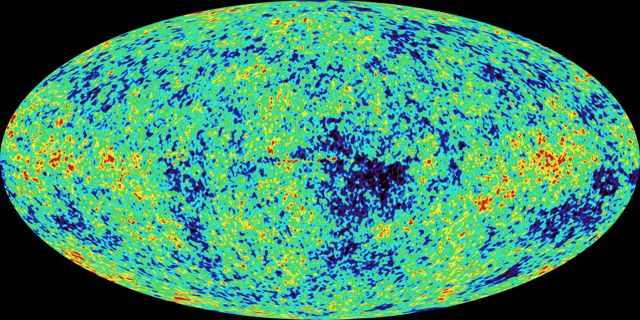
WMapThe picture above shows the latest available all-sky map of fluctuations in the temperature of the cosmic microwave background across the sky as revealed by the Wilkinson Microwave Anisotropy Probe, known to its friends as WMAP.

I’ve spent many long hours fiddling with the data coming from the WMAP experiment, partly because I’ve never quite got over the fact that such wonderful data actually exists. When I started my doctorate in 1985 the whole field of CMB analysis was so much pie in the sky, as no experiments had yet been performed with the sensitivity to reveal the structures we now see. This is because they are very faint and easily buried in noise. The fluctuations in temperature from pixel to pixel across the sky are of order one part in a hundred thousand of the mean temperature (i.e. about 30 microKelvin on a background temperature of about 3 Kelvin). That’s smoother than the surface of a billiard ball. That’s why it took such a long time to make the map shown above, and why it is such a triumphant piece of science.

I blogged a few days ago about the idea that the structure we see in this map was produced by sound waves reverberating around the early Universe. The techniques cosmologists use to analyse this sound are similar to those used in branches of acoustics except that we only see things in projection on the celestial sphere which requires a bit of special consideration.

One of the things that sticks in my brain from my undergraduate years is being told that if a physicist doesn’t know what they are doing they should start by making a Fourier transform. This breaks down the phenomenon being studied into a set of independent plane waves with different wavelengths corresponding to the different tones present in a complicated sound.

It’s often very good advice to do such a decomposition for one-dimensional time series or fluctuation fields in three-dimensional Cartesian space, even you do know what you’re doing, but it doesn’t work with a sphere because plane waves don’t fit properly on a curved surface. Fortunately, however, there is a tried-and-tested alternative involving spherical harmonics rather than plane waves.

Spherical harmonics are quite complicated beasts mathematically but they have pretty similar properties to Fourier harmonics in many respects. In particular they are represented as complex numbers having real and imaginary parts or, equivalently, an amplitude and a phase (usually called an argument by mathematicians). The latter representation is the most useful one for CMB fluctuations because the simplest versions of inflation predict that the phases of each of the spherical harmonic modes should be randomly distributed. What this really means is that there is no information content in their distribution so that the harmonic modes are in a state of maximum statistical disorder or entropy. This property also guarantees that the distribution of fluctuations over the sky should have a Gaussian distribution.

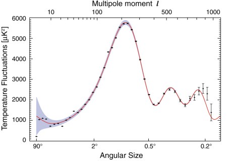
If you accept that the fluctuations are Gaussian then only the amplitudes of the spherical harmonic coefficients are useful. Indeed, their statistical properties can be specified entirely by the variance of these amplitudes as a function of mode frequency. This pre-eminently important function is called the power-spectrum of the fluctuations, and it is shown here for the WMAP data:

080999_powerspectrumm

Although the units on the axes are a bit strange it doesn”t require too much imagination to interpret this in terms of a sound spectrum. There is a characteristic tone (at the position of the peak) plus a couple of overtones. However these features are not sharp so the overall sound is not at all musical.

If the Gaussian assumption is correct then the power-spectrum contains all the useful statistical information to be gleaned from the CMB sky, which is why so much emphasis has been placed on extracting it accurately from the data.

Conversely, though, the power spectrum is completely insenstive to any information in the distribution of spherical harmonic phases. If something beyond the standard model made the Universe non-Gaussian it would affect the phases of the harmonic modes in a way that would make them non-random.

So far, so good. It sounds like it should be a straightforward job to work out whether the WMAP phases are random or not. Unfortunately, though, this task is heavily complicated by the presence of noise and systematics which can be quite easily cleaned from the spectrum but not from more sophisticated descriptors. All we can say so far is that the data seem to be consistent with a Gaussian distribution.

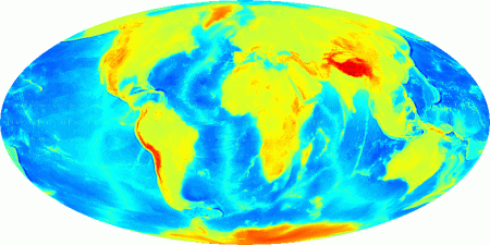
However, I thought I’d end with a bit of fun and show you how important phase information could actually be, if only we could find a good way of exploiting it. Let’s start with a map of the Earth, with the colour representing height of the surface above mean sea level:

sw_world

You can see the major mountain ranges (Andes, Himalayas) quite clearly as red in this picture and note how high Antarctica is…that’s one of the reasons so much astronomy is done there.

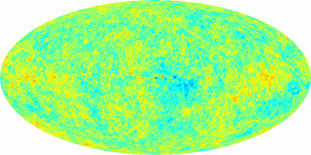
Now, using the same colour scale we have the WMAP data again (in Galactic coordinates).

sw_ilc

The virture of this map is that it shows how smooth the microwave sky is compared to the surface of the Earth. Note also that you can see a bit of crud in the plane of the Milky Way that serves as a reminder of the difficulty of cleaning the foregrounds out.

Clearly these two maps have completely different power spectra. The Earth is dominated by large features made from long-wavelength modes whereas the CMB sky has relatively more small-scale fuzz.

Now I’m going to play with these maps in the following rather peculiar way. First, I make a spherical harmonic transform of each of them. This gives me two sets of complex numbers, one for the Earth and one for WMAP. Following the usual fashion, I think of these as two sets of amplitudes and two sets of phases. Note that the spherical harmonic transformation preserves all the information in the sky maps, it’s just a different representation.

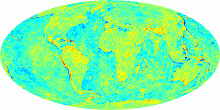
Now what I do is swap the amplitudes and phases for the two maps. First, I take the amplitudes of WMAP and put them with the phases for the Earth. That gives me the spherical harmonic representation of a new data set which I can reveal by doing an inverse spherical transform:

sw_worldphases

This map has exactly the same amplitudes for each mode as the WMAP data and therefore possesses an identical power spectrum to that shown above. Clearly, though, this particular CMB sky is not compatible with the standard cosmological model! Notice that all the strongly localised features such as coastlines appear by virtue of information contained in the phases but absent from the power-spectrum.

To understand this think how sharp features appear in a Fourier transform. A sharp spike at a specific location actually produces a broad spectrum of Fourier modes with different frequencies. These modes have to add in coherently at the location of the spike and cancel out everywhere else, so their phases are strongly correlated. A sea of white noise also has a flat power spectrum but has random phases. The key difference between these two configurations is not revealed by their spectra but by their phases.

Fortunately there is nothing quite as wacky as a picture of the Earth in the real data, but it makes the point that there are more things in Heaven and Earth than can be described in terms of the power spectrum!

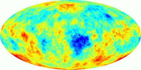
Finally, perhaps in your mind’s eye you might consider what it might look lie to do the reverse experiment: recombine the phases of WMAP with the amplitudes of the Earth.

sw_ilcphases

If the WMAP data are actually Gaussian, then this map is a sort of random-phase realisation of the Earth’s power spectrum. Alternatively you can see that it is the result of running a kind of weird low-pass filter over the WMAP fluctuations. The only striking things it reveals are (i) a big blue hole associated with foreground contamination, (ii) a suspicious excess of red in the galactic plane owing to the same problem, and (iiI) a strong North-South asymmetry arising from the presence of Antarctica.

There’s no great scientific result here, just a proof that spherical harmonics can be fun.

PS. These pictures were made by a former PhD student of mine, Patrick Dineen, who has since quit astronomy to work in high finance. I hope he is weathering the global financial storm!

Misplaced Confidence

Posted in Bad Statistics, The Universe and Stuff with tags , , , on December 10, 2008 by telescoper

From time to time I’ve been posting items about the improper use of statistics. My colleague Ant Whitworth just showed me an astronomical example drawn from his own field of star formation and found in a recent paper by Matthew Bate from the University of Exeter.

The paper is a lengthy and complicated one involving the use of extensive numerical calculations to figure out the effect of radiative feedback on the process of star formation. The theoretical side of this subject is fiendishly difficult, to the extent that it is difficult to make any progress with pencil-and-paper techinques, and Matthew is one of the leading experts in the use of computational methods to tackle problems in this area.

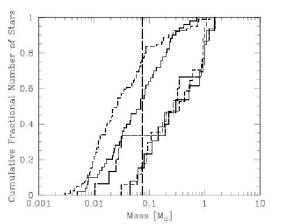
One of the main issues Matthew was investigating was whether radiative feedback had any effect on the initial mass function of the stars in his calculations. The key results are shown in the picture below (Figure 8 from the paper) in terms of cumulative distributions of the star masses in various different situations.

untitled

The question that arises from such data is whether these empirical distributions differ significantly from each other or whether they are consistent with the variations that would naturally arise in different samples drawn from the same distribution. The most interesting ones are the two distributions to the right of the plot that appear to lie almost on top of each other.

Because the samples are very small (only 13 and 15 objects respectively) one can’t reasonably test for goodness-of-fit using the standard chi-squared test because of discreteness effects and because not much is known about the error distribution. To do the statistics, therefore, Matthew uses a popular non-parametric method called the Kolmogorov-Smirnov test which uses the maximum deviation D between the two distributions as a figure of merit to decide whether they match. If D is very large then it is not probable that it can have arisen from the same distribution. If it is smaller then it might have. As for what happens if it is very small then you’ll have to wait a bit.

This is an example of a standard (frequentist) hypothesis test in which the null hypothesis is that the empirical distributions are calculated from independent samples drawn from the same underlying form. The probability of a value of D arising as large as the measured one can be calculated assuming the null is true and is then the significance level of the test. If there’s only a 1% chance of it being as large as the measured value then the significance level is 1%.

So far, so good.

But then, in describing the results of the K-S test the paper states

A Kolmogorov-Smirnov (K-S) test on the …. distributions gives a 99.97% probability that the two IMFs were drawn from the same underlying distribution (i.e. they are statistically indistinguishable).

Agh! No it doesn’t! What it gives is a probability of 99.97% that the chance deviation between the two distributions is expected to be larger than that actually measured. In other words, the two distributions are surprisingly close to each other. But the significance level merely specifies the probability that you would reject the null-hypothesis if it were correct. It says nothing at all about the probability that the null hypothesis is correct. To make that sort of statement you would need to specify an alternative distribution, calculate the distribution of D based on it, and hence determine the statistical power of the test. Without specifying an alternative hypothesis all you can say is that you have failed to reject the null hypothesis.

Or better still, if you have an alternative hypothesis you can forget about power and significance and instead work out the relative probability of the two hypotheses using a proper Bayesian approach.

You might also reasonably ask why might D be so very small? If you find an improbably low value of chi-squared then it usually means either that somebody has cheated or that the data are not independent (which is assumed for the basis of the test). Qualitatively the same thing happens with a KS test.

In fact these two distributions can’t be thought of as independent samples anyway as they are computed from the same initial conditions but with various knobs turned on or off to include different physics. They are not “samples” drawn from the same population but slightly different versions of the same sample. The probability emerging from the KS machinery is therefore meaningless anyway in this context.

So a correct statement of the result would be that the deviation between the two computed distributions is much smaller than one would expect to arise from two independent samples of the same size drawn from the same population.

That’s a much less dramatic statement than is contained in the paper, but has the advantage of not being bollocks.