So how loud was the Big Bang?
I’ve posted on this before but a comment posted today reminded me that perhaps I should recycle it and update it as it relates to the cosmic microwave background, which is what I work on on the rare occasions on which I get to do anything interesting.
As you probably know the Big Bang theory involves the assumption that the entire Universe – not only the matter and energy but also space-time itself – had its origins in a single event a finite time in the past and it has been expanding ever since. The earliest mathematical models of what we now call the Big Bang were derived independently by Alexander Friedman and George Lemaître in the 1920s. The term “Big Bang” was later coined by Fred Hoyle as a derogatory description of an idea he couldn’t stomach, but the phrase caught on. Strictly speaking, though, the Big Bang was a misnomer.
Friedman and Lemaître had made mathematical models of universes that obeyed the Cosmological Principle, i.e. in which the matter was distributed in a completely uniform manner throughout space. Sound consists of oscillating fluctuations in the pressure and density of the medium through which it travels. These are longitudinal “acoustic” waves that involve successive compressions and rarefactions of matter, in other words departures from the purely homogeneous state required by the Cosmological Principle. The Friedman-Lemaitre models contained no sound waves so they did not really describe a Big Bang at all, let alone how loud it was.
However, as I have blogged about before, newer versions of the Big Bang theory do contain a mechanism for generating sound waves in the early Universe and, even more importantly, these waves have now been detected and their properties measured.
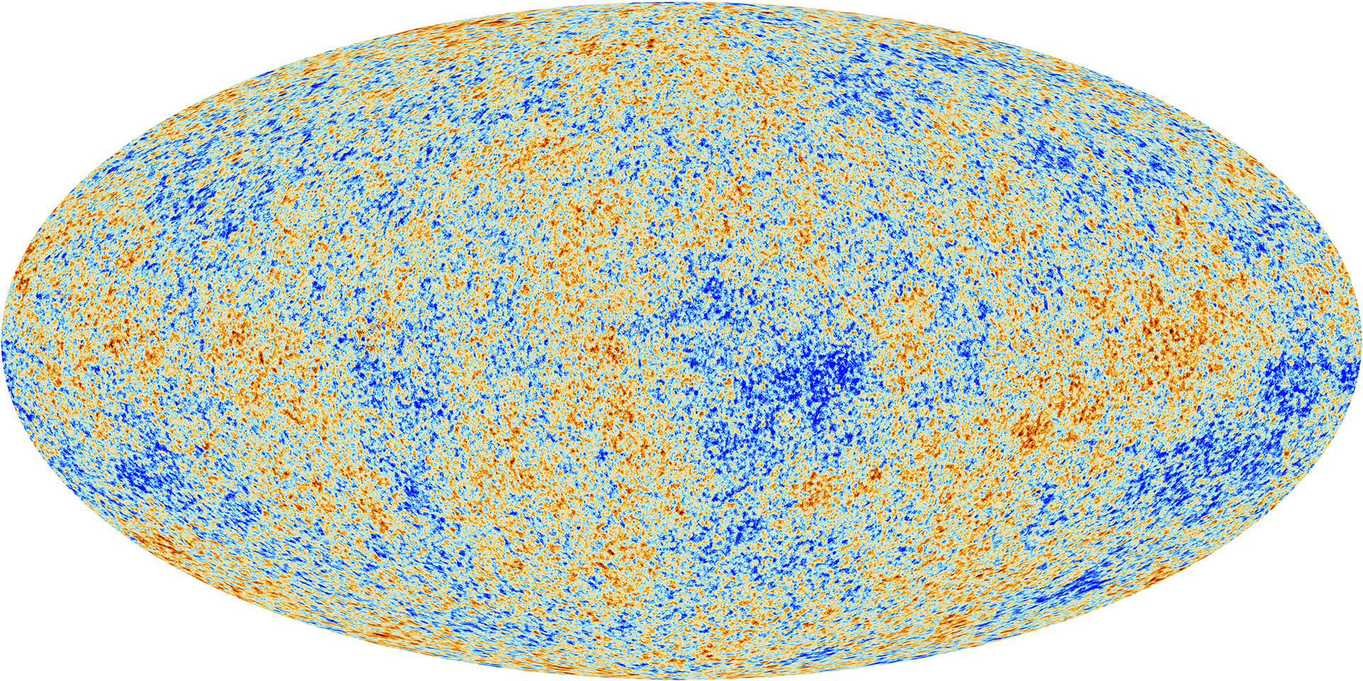
The above image shows the variations in temperature of the cosmic microwave background as charted by the Planck Satellite. The average temperature of the sky is about 2.73 K but there are variations across the sky that have an rms value of about 0.08 milliKelvin. This corresponds to a fractional variation of a few parts in a hundred thousand relative to the mean temperature. It doesn’t sound like much, but this is evidence for the existence of primordial acoustic waves and therefore of a Big Bang with a genuine “Bang” to it.
A full description of what causes these temperature fluctuations would be very complicated but, roughly speaking, the variation in temperature you corresponds directly to variations in density and pressure arising from sound waves.
So how loud was it?
The waves we are dealing with have wavelengths up to about 200,000 light years and the human ear can only actually hear sound waves with wavelengths up to about 17 metres. In any case the Universe was far too hot and dense for there to have been anyone around listening to the cacophony at the time. In some sense, therefore, it wouldn’t have been loud at all because our ears can’t have heard anything.
Setting aside these rather pedantic objections – I’m never one to allow dull realism to get in the way of a good story- we can get a reasonable value for the loudness in terms of the familiar language of decibels. This defines the level of sound (L) logarithmically in terms of the rms pressure level of the sound wave Prms relative to some reference pressure level Pref
L=20 log10[Prms/Pref].
(the 20 appears because of the fact that the energy carried goes as the square of the amplitude of the wave; in terms of energy there would be a factor 10).
There is no absolute scale for loudness because this expression involves the specification of the reference pressure. We have to set this level by analogy with everyday experience. For sound waves in air this is taken to be about 20 microPascals, or about 2×10⁻¹⁰ times the ambient atmospheric air pressure which is about 100,000 Pa. This reference is chosen because the limit of audibility for most people corresponds to pressure variations of this order and these consequently have L=0 dB. It seems reasonable to set the reference pressure of the early Universe to be about the same fraction of the ambient pressure then, i.e.
Pref~2×10⁻¹⁰ Pamb.
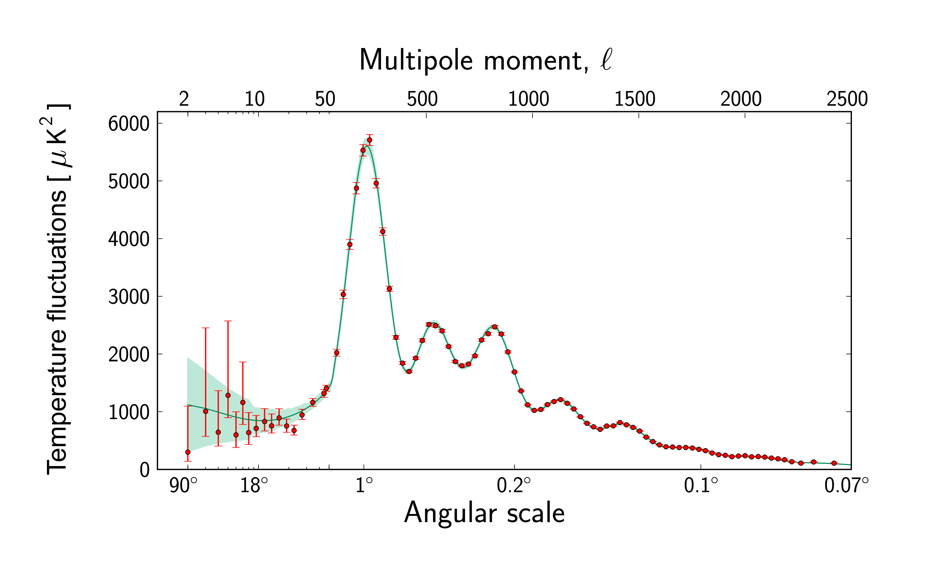
The physics of how primordial variations in pressure translate into observed fluctuations in the CMB temperature is quite complicated, because the primordial universe consists of a plasma rather than air. Moreover, the actual sound of the Big Bang contains a mixture of wavelengths with slightly different amplitudes. In fact here is the spectrum, showing a distinctive signature that looks, at least in this representation, like a fundamental tone and a series of harmonics…
If you take into account all this structure it all gets a bit messy, but it’s quite easy to get a rough but reasonable estimate by ignoring all these complications. We simply take the rms pressure variation to be the same fraction of ambient pressure as the averaged temperature variation are compared to the average CMB temperature, i.e.
Prms~ a few ×10-5Pamb.
If we do this, scaling both pressures in logarithm in the equation in proportion to the ambient pressure, the ambient pressure cancels out in the ratio, which turns out to be a few times 10-5. With our definition of the decibel level we find that waves of this amplitude, i.e. corresponding to variations of one part in a hundred thousand of the reference level, give roughly L=100dB while part in ten thousand gives about L=120dB. The sound of the Big Bang therefore peaks at levels just a bit less than 120 dB.
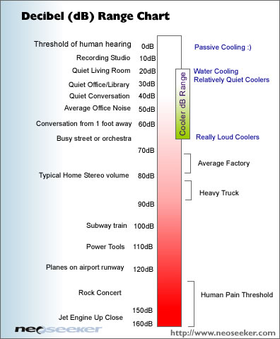
As you can see in the Figure above, this is close to the threshold of pain, but it’s perhaps not as loud as you might have guessed in response to the initial question. Modern popular beat combos often play their dreadful rock music much louder than the Big Bang….
A useful yardstick is the amplitude at which the fluctuations in pressure are comparable to the mean pressure. This would give a factor of about 1010 in the logarithm and is pretty much the limit that sound waves can propagate without distortion. These would have L≈190 dB. It is estimated that the 1883 Krakatoa eruption produced a sound level of about 180 dB at a range of 100 miles. By comparison the Big Bang was little more than a whimper.
PS. If you would like to read more about the actual sound of the Big Bang, have a look at John Cramer’s webpages. You can also download simulations of the actual sound. If you listen to them you will hear that it’s more of a “Roar” than a “Bang” because the sound waves don’t actually originate at a single well-defined event but are excited incoherently all over the Universe.
Follow @telescoper
 of objects of a given mass
  as a function of redshift
  . As an aside, it’s interesting to remark that the
 . But how does that relate to the mass of the halo within which it resides? Clearly the dark matter halo has to be more massive than the baryonic material it collects, and therefore more massive than the central black hole, but by how much?
 for a time order
  years requires a parent halo of mass about
  . Generally, i’s a reasonable back-of-an-envelope estimate that the halo mass would be about a hundred times larger than that of the central black hole so the halo housing this one could be around
  .
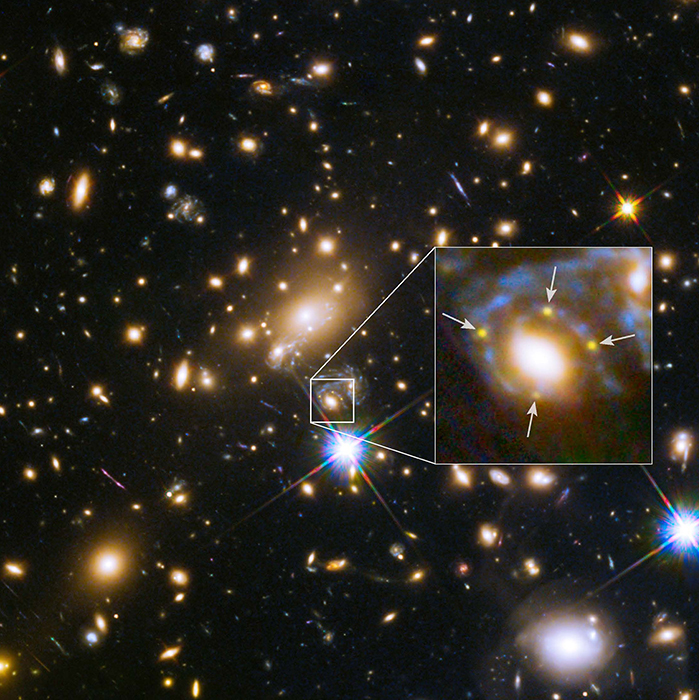
. , are rarer by many orders of magnitude at redshift 7 than at redshift 0 so if anyone ever finds one at this redshift that would really be a shock to many a cosmologist’s system, as would be the discovery of quasars with such a high mass at redshifts significantly higher than seven.


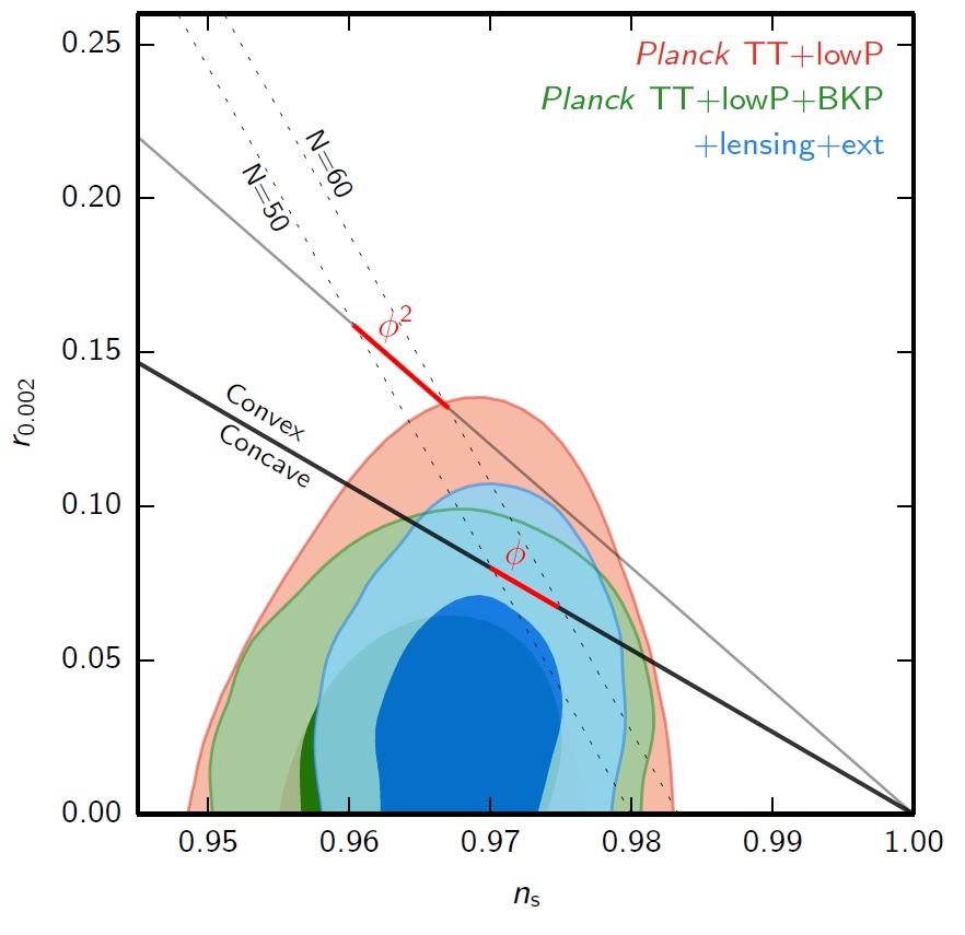
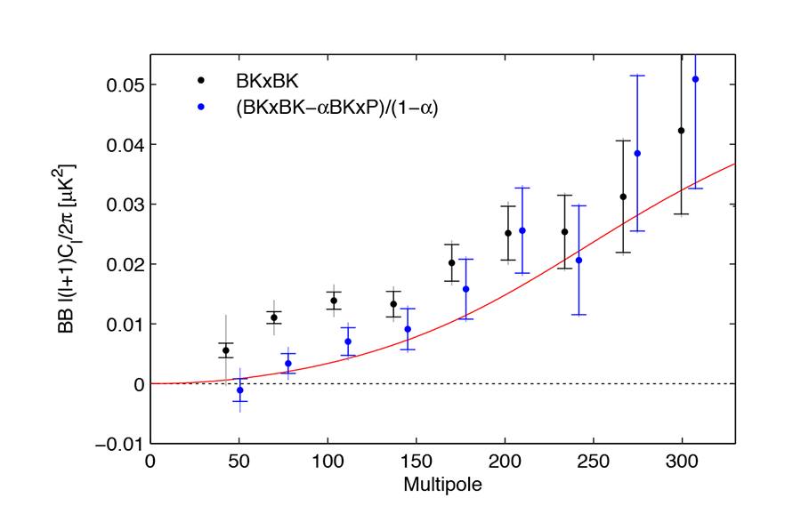
 model of inflation is excluded at greater than 99% confidence…